在 Excel 中根据一个或多个条件提取唯一值
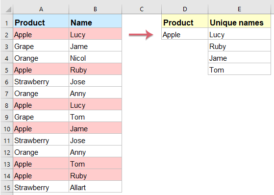
根据条件提取唯一值是数据分析与报表制作中的一项关键任务。假设您左侧有数据区域,希望仅依据 A 列中的特定条件,提取 B 列中的唯一名称。无论您使用的是旧版 Excel,还是 Excel 365/2021 的最新功能,本指南都将为您高效呈现实现方法。
在 Excel 中根据条件提取唯一值
•使用数组公式垂直列出唯一值
要完成此任务,您可以应用一个复杂的数组公式,请按以下步骤操作:
1. 在要显示提取结果的空白单元格中(本例为 E2)输入以下公式,然后按 Shift + Ctrl + Enter 组合键,即可获取第一个唯一值。
=IFERROR(INDEX($B$2:$B$15, MATCH(0, IF($D$2=$A$2:$A$15, COUNTIF($E$1:$E1, $B$2:$B$15), ""), 0)),"")2. 然后向下拖动填充柄,直至出现空白单元格,此时所有符合特定条件的唯一值均已列出,如截图所示:

•使用 Kutools for Excel 在单个单元格中提取并显示唯一值
Kutools for Excel 提供了一种简便方法,无需记忆任何公式,即可将唯一值提取并显示在单个单元格中,助您在处理大型数据集时大幅节省时间和精力。
安装 Kutools for Excel 后,请按以下步骤操作:
单击“Kutools” > “高级 LOOKUP” > “一对多查找(返回多个结果)”以打开对话框。在对话框中,请按以下方式设置操作:
- 分别在文本框中选择“列表放置区域”和“待检索值区域”;
- 选择要使用的表格范围;
- 分别从“关键列”和“返回列”下拉列表中指定关键列和返回列;
- 最后,单击“确定”按钮。


结果:
所有基于条件的唯一名称已提取到单个单元格中,见截图:
•在 Excel 365、Excel 2021 及更高版本中使用公式垂直列出唯一值
在 Excel 365 和 Excel 2021 中,UNIQUE 和 FILTER 等函数让提取唯一值变得前所未有的简单。
将以下公式输入到空白单元格中,然后按 Enter 键,即可一次性垂直获取所有唯一名称。
=UNIQUE(FILTER(B2:B15, A2:A15=D2))
- FILTER(B2:B15, A2:A15=D2):
- FILTER 筛选 B2:B15 区域中的数据。
- A2:A15=D2 检查 A2:A15 中的值是否与 D2 中的值匹配,仅符合条件的行将被包含在结果中。
- UNIQUE(...):
确保仅返回筛选结果中的唯一值。
在 Excel 中根据多个条件提取唯一值
•使用数组公式垂直列出唯一值
如果您希望根据两个条件提取唯一值,以下另一个数组公式可助您一臂之力,请按以下步骤操作:
1. 将以下公式输入到用于列出唯一值的空白单元格中(本例为 G2),然后按 Shift + Ctrl + Enter 组合键,即可获取第一个唯一值。
=IFERROR(INDEX($C$2:$C$15,MATCH(0,COUNTIF(G1:$G$1,$C$2:$C$15)+IF($A$2:$A$15<>$E$2,1,0)+IF($B$2:$B$15<>$F$2,1,0),0)),"")2. 然后向下拖动填充柄,直至出现空白单元格,此时所有符合两个特定条件的唯一值均已列出,详见截图:

•在 Excel 365、Excel 2021 及更高版本中垂直列出唯一值
在新版 Excel 中,根据多个条件提取唯一值要简单得多。
将以下公式输入到空白单元格中,然后按 Enter 键,即可一次性垂直获取所有唯一名称。
=UNIQUE(FILTER(C2:C15, (A2:A15=E2) * (B2:B15=F2)))
- FILTER(C2:C15, (A2:A15=E2) * (B2:B15=F2)):
- FILTER 筛选 C2:C15 范围内的数据。
- (A2:A15=E2) 检查 A 列中的值是否与 E2 单元格中的值匹配。
- (B2:B15=F2) 检查 B 列中的值是否与 F2 单元格中的值匹配。
- *使用 AND 逻辑组合两个条件,仅当两者同时满足时,该行才会被包含在结果中。
- UNIQUE(...):
从筛选结果中剔除重复项,确保输出仅包含唯一值。
使用 Kutools for Excel 从单元格列表中提取唯一值
有时,您可能希望从单元格列表中提取唯一值。这里,我推荐一款实用工具——Kutools for Excel。其“提取区域中唯一值的单元格(包含首个重复项)”功能,可助您快速高效地完成唯一值提取。
1. 单击用于输出结果的单元格。(注意:请勿选择第一行中的单元格。)
2. 然后单击“Kutools”>“公式助手”>“公式助手”,如截图所示:

3. 在“公式助手”对话框中,请执行以下操作:
- 从“公式类型”下拉列表中选择“文本”选项;
- 然后从“选择公式”列表框中选择“提取区域中唯一值的单元格(包含首个重复项)”;
- 在右侧的“参数输入”区域,选择您希望从中提取唯一值的单元格列表。

4. 然后单击“确定”按钮,首个结果将显示在单元格中。接着选中该单元格,向下拖动填充柄,直至出现空白单元格,此时所有唯一值均已列出,见截图:

在 Excel 中根据条件提取唯一值是高效数据分析的一项基本任务,Excel 会根据您的版本和需求提供多种实现方式。选择适合您 Excel 版本和具体需求的方法,即可高效提取唯一值。如果您想掌握更多实用技巧,我们的网站提供数千篇教程,不容错过!
更多相关文章:
- 统计列表中唯一值和不同值的数量
- 假设您有一个包含重复项的长列表,现在希望统计某一列中唯一值(即仅在列表中出现一次的值)或不同值(即列表中所有不重复的值,包括唯一值和首次出现的重复值)的数量,如左图所示。本文将为您介绍如何在 Excel 中轻松完成这一任务。
- 在 Excel 中根据条件对唯一值求和
- 例如,我有一组包含“姓名”和“订单”两列的数据,现在希望根据“姓名”列对“订单”列中的唯一值进行求和,如下图所示。如何在 Excel 中快速轻松地完成这项任务?
- 根据另一列中的唯一值转置一列中的单元格
- 假设您有一组包含两列的数据,现在希望根据另一列中的唯一值,将其中一列的单元格转置为横向排列,从而获得如下所示的结果。您是否知道在 Excel 中实现这一效果的高效方法?
- 在 Excel 中连接唯一值
- 如果我有一个包含重复数据的长列表,现在希望提取唯一值并将它们合并到一个单元格中,如何在 Excel 中快速轻松地实现?
最佳办公效率工具
| 🤖 | KUTOOLS AI 助手:基于以下内容革新数据分析:智能执行 | 生成代码| 创建自定义公式 | 数据分析及生成图表| 调用 Kutools Functions…… |
| 热门功能:查找、高亮或标记重复项 | 删除空白行 | 合并列或单元格且不丢失数据 | 不使用公式的四舍五入…… | |
| 高级 LOOKUP:多条件 VLookup | 多值 VLookup | 跨多工作表 VLookup | 模糊查找…… | |
| 高级下拉列表:快速创建下拉列表 | 级联下拉列表 | 多选下拉列表…… | |
| 列管理器:添加指定数量的列|移动列|切换隐藏列的可见性状态|比较区域与列…… | |
| 特色功能:网格聚焦 | 设计视图 |增强编辑栏 | 工作簿和表管理器 | 资源库(自动文本)| 日期提取 | 汇总工作表 | 加密/解密单元格 | 按列表发送邮件 | 超级筛选 | 特殊筛选(筛选粗体单元格/斜体/删除线……) ...... | |
| 精选 15 工具集:12 文本工具(添加文本,删除特定字符,……)| 50+ 图表 类型(甘特图,……)| 40+ 实用公式(基于生日计算年龄,……)| 19 插入工具(插入二维码,从路径插入图片,……)| 12 转换工具(小写金额转大写,汇率转换,……)| 7 合并和拆分工具(高级合并行,分割单元格,……)|……更多 |
使用 Kutools for Excel 大幅提升您的 Excel 技能,体验前所未有的高效。Kutools for Excel 提供 300 多项高级功能,助您提升生产力、节省时间。立即点击此处,获取您最需要的功能……
Office Tab 为 Office 带来标签式界面,让您的工作更轻松
- 在 Word、Excel、PowerPoint、Publisher、Access、Visio 和 Project 中启用标签式编辑和阅读。
- 在同一个窗口的新标签页中打开并创建多个文档,而非在新窗口中。
- 将您的工作效率提升 50%,每天减少数百次鼠标点击!
所有 Kutools 插件,一个安装程序
Kutools for Office 套件捆绑了适用于 Excel、Word、Outlook 和 PowerPoint 的插件以及 Office Tab Pro,非常适合需要跨多个 Office 应用高效协作的团队。
- 一体化套件— Excel、Word、Outlook 和 PowerPoint 插件 + Office Tab Pro
- 一个安装程序,一个许可证— 几分钟内完成设置(支持 MSI)
- 协同效果更佳— 在多个 Office 应用中实现高效协同
- 30 天全功能试用— 无需注册,无需信用卡
- 超值之选— 比单独购买插件更省钱