在 Excel 中创建搜索框 – 分步指南
在 Excel 中创建搜索框可以更轻松地快速筛选和访问特定数据,从而增强电子表格的功能。本指南涵盖了实现搜索框的几种方法,以适应不同版本的 Excel。无论您是初学者还是高级用户,这些步骤都将帮助您使用 FILTER 函数、条件格式和各种公式等功能设置动态搜索框。
- 轻松创建搜索框 过滤器功能
(适用于 Excel 2019 及更高版本、Excel for Microsoft 365)
- 使用创建搜索框 条件格式
(适用于所有 Excel 版本)
- 创建一个搜索框 配方组合
(适用于所有 Excel 版本)
使用FILTER功能轻松创建搜索框
- 当数据发生变化时,此函数会自动更新输出。
- FILTER 函数可以返回任意数量的结果,从单行到数千行,具体取决于数据集中有多少条目符合您设置的条件。
下面我将向您展示如何使用FILTER函数在Excel中创建搜索框。
步骤1:插入文本框并配置属性
- 去 开发商 标签,点击 插页 > T外部框(ActiveX 控件).
Tips::如果 开发商 选项卡未显示在功能区上,您可以按照本教程中的说明启用它: 如何在Excel功能区中显示/显示开发人员选项卡?

- 光标将变成十字形,然后您需要拖动光标将文本框绘制在工作表中要放置文本框的位置。绘制文本框后,释放鼠标。

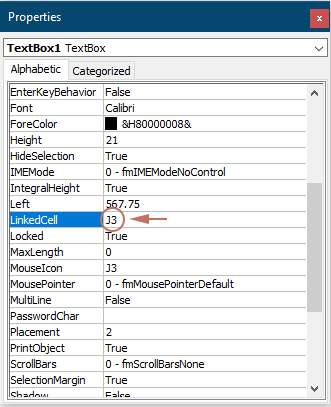
- 右键单击文本框并选择 查看房源 从上下文菜单。

- 在 查看房源 窗格中,通过在文本框中输入单元格引用将文本框链接到单元格 链接单元 场地。例如,输入“J2" 确保在文本框中输入的任何数据都会在单元格 J2 中自动更新,反之亦然。

- 点击 设计模式 在下面 开发商 选项卡退出设计模式。

文本框现在允许您输入文本。
步骤 2:应用 FILTER 功能
- 在使用FILTER功能之前,请将原始标题行复制到新区域。在这里,我将标题行放置在搜索框下方。
Tips::这种方法允许用户在与原始数据相同的列标题下清楚地看到结果。

- 选择第一个标题下的单元格(例如 I5 在此示例中),输入以下公式并按 输入 获得结果的关键。
=FILTER(Sheet2!$A$5:$G$281,Sheet2!$B$5:$B$281=J2,"No data found") 如上面的截图所示,由于文本框现在没有输入,所以公式显示结果“没有找到数据“中 I5.
- 在这个公式中:
- 表 2!$A$5:$G$281:$A$5:$G$281是Sheet2上要过滤的数据范围。
- Sheet2!$B$5:$B$281=J2:这部分定义用于过滤范围的标准。它检查 Sheet5 上第 281 行到第 2 行 B 列中的每个单元格,看看它是否等于单元格 J2 中的值。 J2 是链接到搜索框的单元格。
- 没有找到数据:如果FILTER函数没有找到任何B列中的值等于单元格J2中的值的行,它将返回“未找到数据”。
- 这个方法是 不区分大小写,这意味着无论您输入大写字母还是小写字母,它都会匹配文本。
结果:测试搜索框
现在让我们测试一下搜索框。在这个例子中,当我在搜索框中输入客户姓名时,相应的结果将立即被过滤并显示。

使用条件格式创建搜索框
条件格式可用于突出显示与搜索词匹配的数据,从而间接创建搜索框效果。此方法不会过滤掉数据,而是直观地引导您找到相关单元格。本节将向您展示如何使用 Excel 中的条件格式创建搜索框。
步骤1:插入文本框并配置属性
- 去 开发商 标签,点击 插页 > T外部框(ActiveX 控件).
Tips::如果 开发商 选项卡未显示在功能区上,您可以按照本教程中的说明启用它: 如何在Excel功能区中显示/显示开发人员选项卡?
- 光标将变成十字形,然后您需要拖动光标将文本框绘制在工作表中要放置文本框的位置。绘制文本框后,释放鼠标。
- 右键单击文本框并选择 查看房源 从上下文菜单。
- 在 查看房源 窗格中,通过在文本框中输入单元格引用将文本框链接到单元格 链接单元 场地。例如,输入“J3" 确保在文本框中输入的任何数据都会在单元格 J3 中自动更新,反之亦然。
- 点击 设计模式 在下面 开发商 选项卡退出设计模式。
文本框现在允许您输入文本。
步骤 2:应用条件格式来搜索数据
- 选择要搜索的整个数据范围。这里我选择范围A3:G279。
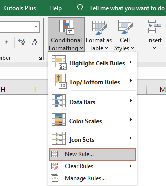
- 在下面 主页 标签,点击 条件格式 > 新规则.
- 在 新格式规则 对话框:
- 选择 使用公式来确定要格式化的单元格 ,在 选择规则类型 选项。
- 将以下公式输入到 格式化此公式为真的值 框。
=$B3=$J$3在这里, $ B3 表示要与选定范围内的搜索条件匹配的列中的第一个单元格,以及 $J$3 是链接到搜索框的单元格。 - 点击 格式 按钮指定搜索结果的填充颜色。
- 点击 OK 按钮。 看截图:

结果
现在让我们测试一下搜索框。在此示例中,当我在搜索框中输入客户姓名时,B 列中包含该客户的相应行将立即使用指定的填充颜色突出显示。
创建包含公式组合的搜索框
如果您没有使用最新版本的 Excel 并且不希望仅突出显示行,本节中描述的方法可能会有所帮助。您可以使用 Excel 公式的组合在任何版本的 Excel 中创建功能搜索框。请按照以下步骤操作。
步骤 1:从搜索列创建唯一值列表
- 在本例中,我选择并复制范围 B4:B281 到一个新的工作表。
- 将范围粘贴到新工作表中后,保持所选粘贴的数据,转到 时间 选项卡,并选择 删除重复.

- 在开幕 删除重复 对话框中,单击 OK 按钮。
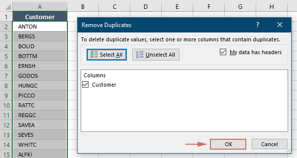
- A 微软的Excel 然后弹出提示框,显示删除了多少重复项。点击 OK.

- 删除重复项后,选择列表中的所有唯一值(不包括标题),并通过在 名字 盒子。这里我将范围命名为 对客户的.

步骤 2:插入组合框并配置属性
- 返回到包含要搜索的数据集的工作表。前往 开发商 标签,点击 插页 > 组合框(ActiveX控件).
Tips::如果 开发商 选项卡未显示在功能区上,您可以按照本教程中的说明启用它: 如何在Excel功能区中显示/显示开发人员选项卡?

- 光标将变成十字形,然后您需要拖动光标在工作表中要放置搜索框的位置绘制组合框。绘制组合框后,释放鼠标。
- 右键单击组合框并选择 查看房源 从上下文菜单。

- 在 查看房源 窗格:
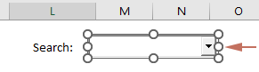
- 通过在单元格引用中输入单元格引用,将组合框链接到单元格 链接单元 场地。她我输入“M2".
提示:指定此字段可确保在组合框中输入的任何数据都将在单元格 M2 中自动更新,反之亦然。
- 在 列表填充范围 字段,输入 范围名称 您在步骤 1 中指定了唯一列表。
- 更改 匹配项 字段 2 – fmMatchEntryNone.
- 关上 查看房源 窗格。
- 通过在单元格引用中输入单元格引用,将组合框链接到单元格 链接单元 场地。她我输入“M2".
- 点击 设计模式 在下面 开发商 选项卡退出设计模式。
您现在可以从组合框中选择任何项目或输入要搜索的文本。
第 3 步:应用公式
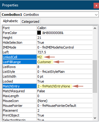
- 创建与原始数据范围相邻的三个辅助列。看截图:

- 在单元格中(H5)在第一个辅助列的标题下,输入以下公式并按 输入.
=ROWS($B$5:B5)这里 B5 是包含要搜索的列的第一个客户名称的单元格。
- 双击右下角的公式单元格,后面的单元格会自动填写相同的公式。
- 在单元格中(I5)在第二个辅助列标题下,输入以下公式并按 输入。然后双击公式单元格的右下角,自动用相同的公式填充下面的单元格。
=IF(ISNUMBER(SEARCH($M$2,B5)),H5,"")这里 M2 是链接到组合框的单元格。
- 在单元格中(J5)在第三个辅助列标题下,输入以下公式并按 输入。然后双击公式单元格的右下角,自动用相同的公式填充下面的单元格。
=IFERROR(SMALL($I$5:$I$281,H5),"")
- 将原始标题行复制到新区域。在这里,我将标题行放置在搜索框下方。
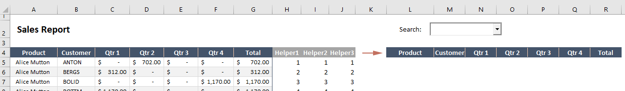
- 选择第一个标题下的单元格(例如 L5 在本例中),输入以下公式并按 Enter 键。
=IFERROR(INDEX($A$5:$G$281,$J5,COLUMNS($L$4:L4)),"")这里 A5:G281 是您想要在结果单元格中显示的整个数据范围。
- 选择该公式单元格,拖动 填充手柄 向右然后向下将公式应用到相应的列和行。
 :
:- 由于搜索框中没有输入,公式的结果将显示原始数据。
- 此方法不区分大小写,这意味着无论您输入大写字母还是小写字母,它都会匹配文本。
结果
现在让我们测试一下搜索框。在此示例中,当我从组合框中输入或选择客户名称时,B 列中包含该客户名称的相应行将被过滤并立即显示在结果范围中。

在 Excel 中创建搜索框可以显着改善您与数据的交互方式,使您的电子表格更加动态且用户友好。无论您选择简单的 FILTER 函数、条件格式的视觉辅助,还是选择多功能的公式组合,每种方法都提供了宝贵的工具来增强您的数据操作能力。尝试这些技术,找出最适合您的特定需求和数据场景的技术。对于那些渴望深入研究 Excel 功能的人,我们的网站拥有丰富的教程。 在这里了解更多 Excel 提示和技巧.
最佳办公生产力工具
| 🤖 | Kutools 人工智能助手:基于以下内容彻底改变数据分析: 智能执行 | 生成代码 | 创建自定义公式 | 分析数据并生成图表 | 调用 Kutools 函数... |
| 热门特色: 查找、突出显示或识别重复项 | 删除空白行 | 合并列或单元格而不丢失数据 | 不使用公式进行四舍五入 ... | |
| 超级查询: 多条件VLookup | 多值VLookup | 跨多个工作表的 VLookup | 模糊查询 .... | |
| 高级下拉列表: 快速创建下拉列表 | 依赖下拉列表 | 多选下拉列表 .... | |
| 列管理器: 添加特定数量的列 | 移动列 | 切换隐藏列的可见性状态 | 比较范围和列 ... | |
| 特色功能: 网格焦点 | 设计图 | 大方程式酒吧 | 工作簿和工作表管理器 | 资源库 (自动文本) | 日期选择器 | 合并工作表 | 加密/解密单元格 | 按列表发送电子邮件 | 超级筛选 | 特殊过滤器 (过滤粗体/斜体/删除线...)... | |
| 前 15 个工具集: 12 文本 工具 (添加文本, 删除字符,...) | 50+ 图表 类型 (甘特图,...) | 40+ 实用 公式 (根据生日计算年龄,...) | 19 插入 工具 (插入二维码, 从路径插入图片,...) | 12 转化 工具 (小写金额转大写, 货币兑换,...) | 7 合并与拆分 工具 (高级组合行, 分裂细胞,...) | ... 和更多 |
使用 Kutools for Excel 增强您的 Excel 技能,体验前所未有的效率。 Kutools for Excel 提供了 300 多种高级功能来提高生产力并节省时间。 单击此处获取您最需要的功能...
")
Office Tab 为 Office 带来选项卡式界面,让您的工作更加轻松
- 在Word,Excel,PowerPoint中启用选项卡式编辑和阅读,发布者,Access,Visio和Project。
- 在同一窗口的新选项卡中而不是在新窗口中打开并创建多个文档。
- 每天将您的工作效率提高50%,并减少数百次鼠标单击!
")