跳到主要内容

如何在Excel中基于多个条件计算唯一值?

本文,我将为您提供一些示例,供您根据工作表中的一个或多个条件来计算唯一值。 以下详细步骤可能会对您有所帮助。

根据一项标准计算唯一值

根据两个给定日期计算唯一值

根据两个条件计算唯一值

根据三个条件计算唯一值


箭头蓝色右气泡 根据一项标准计算唯一值

例如,我有以下数据范围,现在,我要计算汤姆销售的独特产品。

具有多个条件的唯一文档数1

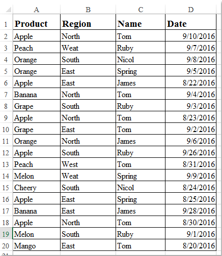
请将此公式输入到要获取结果的空白单元格中,例如G2:

= SUM(IF(“ Tom” = $ C $ 2:$ C $ 20,1 /(COUNTIFS($ C $ 2:$ C $ 20,“ Tom”,$ A $ 2:$ A $ 20,$ A $ 2:$ A $ 20) ),0)),然后按 Shift + Ctrl + 输入 键在一起以获得正确的结果,请参见屏幕截图:

具有多个条件的唯一文档数2

备注:在上式中,“Tom”是您要依据的名称标准, C2:C20 是包含名称标准的单元格 A2:A20 是您要计算唯一值的单元格。


箭头蓝色右气泡 根据两个给定日期计算唯一值

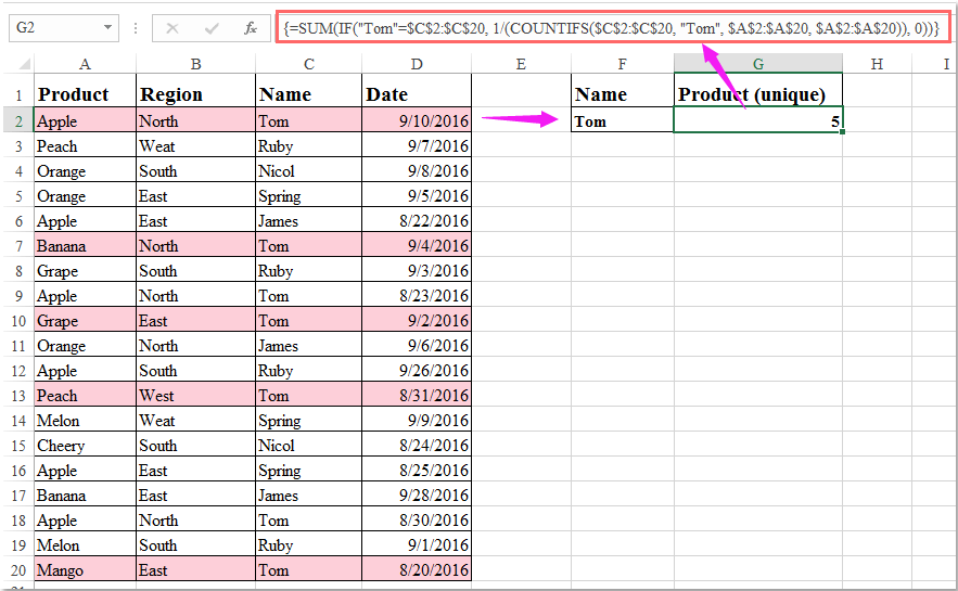
要计算两个给定日期之间的唯一值,例如,我要计算日期范围2016/9/1和2016/9/30之间的唯一乘积,请应用以下公式:

= SUM(IF($ D $ 2:$ D $ 20 <= DATE(2016,9,30)*($ D $ 2:$ D $ 20> = DATE(2016,9,1))),1 / COUNTIFS($ A $ 2 :$ A $ 20,$ A $ 2:$ A $ 20,$ D $ 2:$ D $ 20,“ <=”&DATE(2016,9,30),$ D $ 2:$ D $ 20,“> =”&DATE(2016, 9,1))),0),然后按 Shift + Ctrl + 输入 键一起获得唯一的结果,请参见屏幕截图:

具有多个条件的唯一文档数3

备注:在上式中,日期 2016,9,12016,9,30 是您要计算的开始日期和结束日期, D2:D20 单元格是否包含日期条件, A2:A20 是要从中计算唯一值的单元格。


箭头蓝色右气泡 根据两个条件计算唯一值

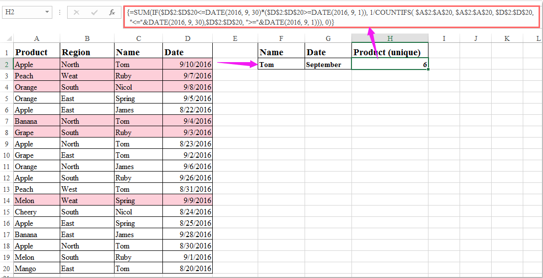
如果您要计算汤姆XNUMX月份销售的独特产品,以下公式可以为您提供帮助。

请将此公式输入空白单元格以输出结果,例如H2。

= SUM(IF((“ Tom” = $ C $ 2:$ C $ 20)*($ D $ 2:$ D $ 20 <= DATE(2016,9,30)*($ D $ 2:$ D $ 20> = DATE( 2016,9,1))))/ 1 / COUNTIFS($ C $ 2:$ C $ 20,“ Tom”,$ A $ 2:$ A $ 20,$ A $ 2:$ A $ 20,$ D $ 2:$ D $ 20,“ <=“&DATE(2016,9,30),$ D $ 2:$ D $ 20,”> =“&DATE(2016,9,1))),0) 然后按 Shift + Ctrl + 输入 键一起获得唯一的结果,请参见屏幕截图:

具有多个条件的唯一文档数4

笔记:

1.在上式中,“Tom”是名称标准, 2016,9,12016,9,30 是您要基于的两个日期, C2:C20 是单元格包含名称标准,并且 D2:D20 单元格中是否包含日期, A2:A20 是您要计算唯一值的单元格范围。

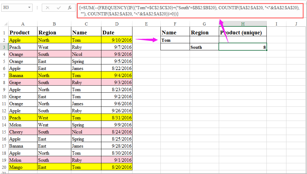
2.如果您需要使用“or”来计算唯一值的标准,例如,计算汤姆或在南部地区销售的产品,请应用以下公式:

=SUM(--(FREQUENCY(IF(("Tom"=$C$2:$C$20)+("South"=$B$2:$B$20), COUNTIF($A$2:$A$20, "<"&$A$2:$A$20), ""), COUNTIF($A$2:$A$20, "<"&$A$2:$A$20))>0)),并记得按 Shift + Ctrl + 输入 键一起获得唯一的结果,请参见屏幕截图:

具有多个条件的唯一文档数5


箭头蓝色右气泡 根据三个条件计算唯一值

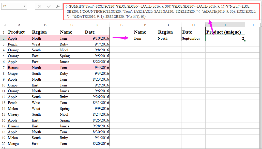
要用三个标准来计算唯一产品,公式可能会更复杂。 假设计算出汤姆(Tom)在XNUMX月份和北部地区销售的独特产品。 请这样做:

将此公式输入空白单元格以输出结果I2,例如:

= SUM(IF((“ Tom” = $ C $ 2:$ C $ 20)*($ D $ 2:$ D $ 20 <= DATE(2016,9,30))*($ D $ 2:$ D $ 20> = DATE (2016,9,1))*(“北” = $ B $ 2:$ B $ 20),1 / COUNTIFS($ C $ 2:$ C $ 20,“ Tom”,$ A $ 2:$ A $ 20,$ A $ 2 :$ A $ 20,$ D $ 2:$ D $ 20,“ <=”&DATE(2016,9,30),$ D $ 2:$ D $ 20,“> =”&DATE(2016,9,1),$ B $ 2 :$ B $ 20,“北”)),0),然后按 Shift + Ctrl + 输入 键一起获得唯一的结果,请参见屏幕截图:

具有多个条件的唯一文档数6

最佳办公生产力工具

🤖 Kutools 人工智能助手:基于以下内容彻底改变数据分析: 智能执行   |  生成代码  |  创建自定义公式  |  分析数据并生成图表  |  调用 Kutools 函数...
热门特色: 查找、突出显示或识别重复项   |  删除空白行   |  合并列或单元格而不丢失数据   |   不使用公式进行四舍五入 ...
超级查询: 多条件VLookup    多值VLookup  |   跨多个工作表的 VLookup   |   模糊查询 ....
高级下拉列表: 快速创建下拉列表   |  依赖下拉列表   |  多选下拉列表 ....
列管理器: 添加特定数量的列  |  移动列  |  切换隐藏列的可见性状态  |  比较范围和列 ...
特色功能: 网格焦点   |  设计图   |   大方程式酒吧    工作簿和工作表管理器   |  资源库 (自动文本)   |  日期选择器   |  合并工作表   |  加密/解密单元格    按列表发送电子邮件   |  超级筛选   |   特殊过滤器 (过滤粗体/斜体/删除线...)...
前 15 个工具集12 文本 工具 (添加文本, 删除字符,...)   |   50+ 图表 类型 (甘特图,...)   |   40+ 实用 公式 (根据生日计算年龄,...)   |   19 插入 工具 (插入二维码, 从路径插入图片,...)   |   12 转化 工具 (小写金额转大写, 货币兑换,...)   |   7 合并与拆分 工具 (高级组合行, 分裂细胞,...)   |   ... 和更多

使用 Kutools for Excel 增强您的 Excel 技能,体验前所未有的效率。 Kutools for Excel 提供了 300 多种高级功能来提高生产力并节省时间。  单击此处获取您最需要的功能...

产品描述


Office Tab 为 Office 带来选项卡式界面,让您的工作更加轻松

  • 在Word,Excel,PowerPoint中启用选项卡式编辑和阅读,发布者,Access,Visio和Project。
  • 在同一窗口的新选项卡中而不是在新窗口中打开并创建多个文档。
  • 每天将您的工作效率提高50%,并减少数百次鼠标单击!
Comments (19)
No ratings yet. Be the first to rate!
This comment was minimized by the moderator on the site
For all the above formula an you suggest a non array formula as my data runs to 25000 rows. I need a free suggestions and not paid ones
This comment was minimized by the moderator on the site
Hi,
This is great - except I cant get it to work for what I require
I have two sheets - a Summary sheet, and another sheet containing data
The dates are dynamic - so you enter the date ranges in the Summary sheet in two cells (from B2 to D2)
When I replace DATE(2022,6,1) with B2 it comes back with "a value used in the formula is the wrong data type"
When I test with putting DATE(2022,6,1) and DATE (2022,6,30) in the from - to parts in the formula - I get 0 as the result - which is wrong.
Note: I'm in Ireland - so the date format here is dd.mm.yy - changing things doesn't fix - and adds confusion tbh
My formula is
=SUM(IF(Sheet4!$C$2:Sheet4!$C$65<=(D2)*(Sheet4!$C$2:Sheet4!$C$65>=(B2)), 1/COUNTIFS(Sheet4!$A$2:Sheet4!$A$65, Sheet4!$A$2:Sheet4!$A$65, Sheet4!$C$2:Sheet4!$C$65, "<="&D2,Sheet4!$C$2:Sheet4!$C$65, ">="&B2))),0)
Where Sheet4 contains the data, C2:C65 are cells with dates, A2:A65 are cells with project numbers - where there maybe duplicates
Any help - greatly appreciated,
Thanks
This comment was minimized by the moderator on the site
1 month2 brand name 3 executive wise4 mix party nameCount unique party name
This comment was minimized by the moderator on the site
Count Unique Values Based On four Criteria
This comment was minimized by the moderator on the site
I am trying to use this method to calculate unique customers for a particular product (where a customer may have bought multiple times, but I want unique customers). If I enter the formula but limit the range to a subset of just 5 rows that I know contain a duplicate customer, it works fine. But when I apply to the whole column, e.g. $D:$D, it calculates endlessly; if it finishes, it returns a wrong result. But now it's not even finishing and I have to end the Excel process. Is this just too costly in terms of CPU to apply to a large volume of data (e.g. 1500 rows)?
This comment was minimized by the moderator on the site
I ma getting value in point which is not possible So please help me Out

{=SUM(IF(("Regular"='Raw Data'!$G$5:$G$1785)*('Raw Data'!$D$5:$D$1785<=DATE(2019,6,30)*('Raw Data'!$D$5:$D$1785>=DATE(2019,6,1))),1/COUNTIFS('Raw Data'!$B$5:$B$1785,'Raw Data'!$B$5:$B$1785,'Raw Data'!$D$5:$D$1785,"<="&DATE(2019,6,30),'Raw Data'!$D$5:$D$1785,">="&DATE(2019,6,1))),0)}
This comment was minimized by the moderator on the site
my question.
I mean that filtered rows , and not count hidden rows.
This comment was minimized by the moderator on the site
"if count visible rows."
I mean filtered rows , and not count rows hidden.
This comment was minimized by the moderator on the site
Ffrom this article formula,
if count visible rows. how can add or edit formula?
This comment was minimized by the moderator on the site
The greater and less than date criteria is a distracting example of how to use the sumif array.
There are no comments posted here yet
Load More
Please leave your comments in English
Posting as Guest
×
Rate this post:
0   Characters
Suggested Locations