跳到主要内容

如何基于Excel中的单元格值在单元格中动态插入图像或图片?

在许多情况下,您可能需要根据单元格值在单元格中动态插入图像。 例如,您希望使用您在指定单元格中输入的不同值动态更改相应的图像。 本文将向您展示如何实现它。

根据您在单元格中输入的值动态插入和更改图像
使用惊人的工具根据单元格值动态更改图像


根据您在单元格中输入的值动态插入和更改图像

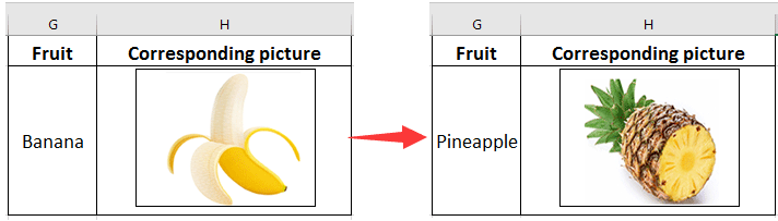
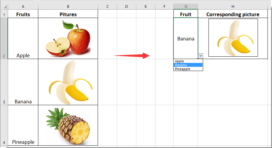
如下面的屏幕截图所示,您要基于在单元格G2中输入的值动态显示相应的图片。 在单元格G2中输入“香蕉”时,香蕉图片将显示在单元格H2中。 在单元格G2中输入菠萝时,单元格H2中的图片将变成相应的菠萝图片。

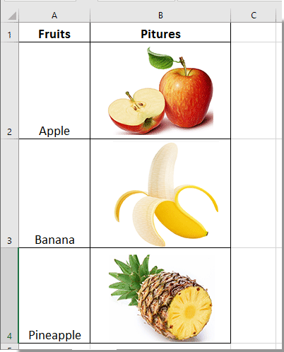
1.在工作表中创建两列,第一列范围 A2:A4 包含图片名称和第二列范围 B2:B4 包含相应的图片。 请参阅显示的屏幕截图。
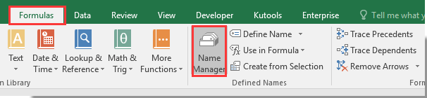
2。 点击 公式 > 名称管理员.

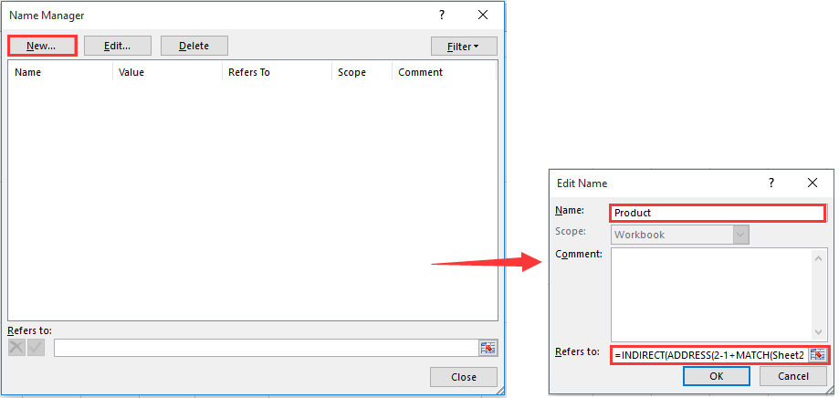
3.在 名称管理员 对话框中,单击 全新 按钮。 然后 编辑名称 弹出对话框,输入 产品 名字 框中,将以下公式输入 框,然后单击 OK 按钮。 看截图:

=INDIRECT(ADDRESS(2-1+MATCH(Sheet2!$G$2, Sheet2!$A$2:$A$4, 0), 2))

:

1)。 在公式中,第一个数字 2 是您的第一个产品的行号。 在这种情况下,我的第一个产品名称位于第2行。
2)。 Sheet2!$ G $ 2 是您要基于其动态更改相应图像的单元格。
3)。 Sheet2!$ A $ 2:$ A $ 4 是您在当前工作表中的产品名称列表。
4)。 最后一个号码 2 是包含您的图像的列号。

您可以根据需要在上述公式中更改它们。

4.关闭 名称管理员 对话框。

5.在“图片”列中选择一张图片,然后按 按Ctrl + C 同时复制键。 然后将其粘贴到当前工作表中的新位置。 在这里,我复制苹果图片并将其放在单元格H2中。

6.在单元格G2中输入一个水果名称(例如Apple),单击以选择粘贴的图片,然后输入公式 =产品配方栏,然后按 输入 键。 看截图:

从现在开始,当更改为G2单元格中的任何水果名称时,H2单元格中的图片将动态变为对应的水果名称。

您可以通过在G2单元格中创建一个包含所有水果名称的下拉列表来快速选择水果名称,如下图所示。


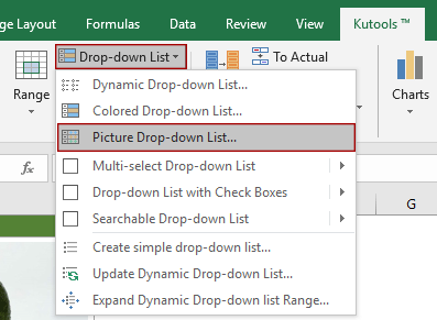
使用惊人的工具根据单元格值轻松将图像插入相关单元格

对于很多Excel新手来说,上面的方法并不好驾驭。 这里推荐 图片下拉列表 的特点 Kutools for Excel. 使用此功能,您可以轻松创建值和图片完全匹配的动态下拉列表。

申请前 Kutools for Excel首先下载并安装.

请按照以下步骤应用Kutools for Excel的图片下拉列表功能在Excel中创建动态图片下拉列表。

1.首先,您需要分别创建两列,分别包含值及其对应的图片,如下图所示。

2。 点击 库工具 > 进出口 > 匹配导入图片.

3.在 图片下拉列表 对话框,您需要配置如下。

3.1) 如果您已经在上面的步骤 1 中创建了值和图片列,请忽略此步骤;
3.2)在 Step2 部分,选择您创建的两列;
3.3)在 Step3 部分,选择输出动态图片的范围下拉列表。
请注意: In Step3 部分,您需要选择两列来放置结果。 一列用于值,另一列用于相应的图片。
3.4)点击 确定。

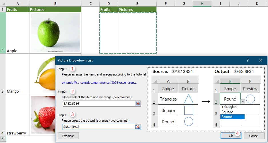
4.然后 Kutools for Excel 弹出对话框提醒您在此过程中会创建一些中间数据,点击 USB MIDI(XNUMX通道) 继续。

然后创建一个动态图片下拉列表。 图片将根据您在下拉列表中选择的项目动态更改。

点击 了解有关此功能的更多信息...

  如果您想免费试用(30天)此实用程序, 请点击下载,然后按照上述步骤进行操作。


相关文章:

最佳办公生产力工具

🤖 Kutools 人工智能助手:基于以下内容彻底改变数据分析: 智能执行   |  生成代码  |  创建自定义公式  |  分析数据并生成图表  |  调用 Kutools 函数...
热门特色: 查找、突出显示或识别重复项   |  删除空白行   |  合并列或单元格而不丢失数据   |   不使用公式进行四舍五入 ...
超级查询: 多条件VLookup    多值VLookup  |   跨多个工作表的 VLookup   |   模糊查询 ....
高级下拉列表: 快速创建下拉列表   |  依赖下拉列表   |  多选下拉列表 ....
列管理器: 添加特定数量的列  |  移动列  |  切换隐藏列的可见性状态  |  比较范围和列 ...
特色功能: 网格焦点   |  设计图   |   大方程式酒吧    工作簿和工作表管理器   |  资源库 (自动文本)   |  日期选择器   |  合并工作表   |  加密/解密单元格    按列表发送电子邮件   |  超级筛选   |   特殊过滤器 (过滤粗体/斜体/删除线...)...
前 15 个工具集12 文本 工具 (添加文本, 删除字符,...)   |   50+ 图表 类型 (甘特图,...)   |   40+ 实用 公式 (根据生日计算年龄,...)   |   19 插入 工具 (插入二维码, 从路径插入图片,...)   |   12 转化 工具 (小写金额转大写, 货币兑换,...)   |   7 合并与拆分 工具 (高级组合行, 分裂细胞,...)   |   ... 和更多

使用 Kutools for Excel 增强您的 Excel 技能,体验前所未有的效率。 Kutools for Excel 提供了 300 多种高级功能来提高生产力并节省时间。  单击此处获取您最需要的功能...

产品描述


Office Tab 为 Office 带来选项卡式界面,让您的工作更加轻松

  • 在Word,Excel,PowerPoint中启用选项卡式编辑和阅读,发布者,Access,Visio和Project。
  • 在同一窗口的新选项卡中而不是在新窗口中打开并创建多个文档。
  • 每天将您的工作效率提高50%,并减少数百次鼠标单击!
Comments (15)
No ratings yet. Be the first to rate!
This comment was minimized by the moderator on the site
Can this be paired up with excel Queries?
This comment was minimized by the moderator on the site
Hi Maxem,
The methods can't be paired up with Excel queries, and I have not been able to fix the problem. Sorry for the inconvenience.
This comment was minimized by the moderator on the site
What if the cell value we take to change the picture has more than one word. Like a company name and logo
This comment was minimized by the moderator on the site
How can I, if no value is entered, reset to a defaut image (or nothing)?Thanks
This comment was minimized by the moderator on the site
Hi Admin
Thanks for sharing very good article. Could you please tell me, In Ist procedure step 6, I want to enter value for G2 through a user form. Is it possible? Please help
This comment was minimized by the moderator on the site
Good day,
Sorry, the user form does not take into consideration in this case.
This comment was minimized by the moderator on the site
Could this be used instead of conditional formatting icon sets?
I need a green down arrow and red up arrow based on percentages from other cells.


If so, how would I go about completing this?

I'm needing negative percentages (<0%) to show a red up arrow,
Neutral percentages (=0%) to show a yellow bracket. (can already be done with conditional formatting),
Positive percentages (>=0.001%) to show a green down arrow.


How would I achieve this?
This comment was minimized by the moderator on the site
Dear Jason,
Sorry i don't have methd for this question.
This comment was minimized by the moderator on the site
Looks really great! But I need it to auto fill a cell (B1) with a picture when I type something in cell A1. Is this possible? and can we change max file count in folder? Have one with 15.000 pics, max is 10000.

Thanks! Love to hear from you@!
This comment was minimized by the moderator on the site
Guido, the problem you mentioned cannot be solved. Sorry about that!
This comment was minimized by the moderator on the site
Can you please tell, how can this be looped for over 600 rows. Here in this tutorial, it changes picture based on only one cell, I need the same for multiple cells, do I need to make separate "Product" lists for that in "Name Manager", because that lists is over 600.
This comment was minimized by the moderator on the site
Dear Nick,

Sorry to tell you that this method can't be looped for multiple cells. You need to specify =Product formula to all needed pictures one by one manually in your case.
Thank you for your comment!
This comment was minimized by the moderator on the site
This is awesome, is there a way of creating a lookup formula on another worksheet that will look up the name and return the picture into the selected cell?
This comment was minimized by the moderator on the site
Hey Nick did you get how to do it, when you want to have the list of the pictures on other sheet?
This comment was minimized by the moderator on the site
Great article, really helpful for something I'm trying to do. How would you change the formula in step 3 if all of the images and names were on another worksheet? Many thanks.
There are no comments posted here yet
Please leave your comments in English
Posting as Guest
×
Rate this post:
0   Characters
Suggested Locations