如何VLOOKUP最小值并返回Excel中的相邻单元格？

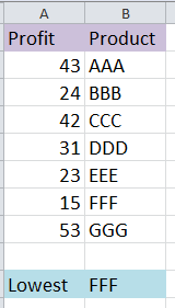
如果您有一系列数据，并且想要在A列中找到最低值，然后在B列中返回其相邻的单元格，如下面的屏幕截图所示，那么如何快速解决它而不是一个一个地找到它？ VLOOKUP函数非常强大，可以轻松解决此问题，现在我将讨论使用VLOOKUP查找最小值并返回Excel中的相邻单元格。
VLOOKUP最小值并返回相邻单元格
索引最小值并返回相邻单元格

VLOOKUP最小值并返回相邻单元格

在这里，我告诉您一个VLOOKUP公式以查找最小值并返回相邻的单元格。

选择要放入结果的单元格，然后键入此公式 = VLOOKUP（MIN（$ A $ 2：$ A $ 8），$ A $ 2：$ B $ 8，2，0），然后按 输入 键，然后您将相邻单元格设置为最低值。

请注意：

1. A2：A8是要查找最小值的范围，A2：B8是数据的范围。

2.使用VLOOKUP功能，您只能返回右列中的相邻单元格。

3.如果您要查找的最低值列中的最低值重复，则此公式将返回相邻的第一最低值的单元格。

索引最小值并返回相邻单元格

为了找到最小值并使用VLOOKUP返回相邻单元格有一些限制，现在我介绍INDEX函数来解决此问题。

选择一个您想要使相邻单元格达到最小值的单元格，然后键入此公式 =INDEX(A2:A8,MATCH(MIN(B2:B8),B2:B8,0))，然后按 输入 键。 看截图：

请注意：

1. A2：A8是包含要返回的单元格的范围，B2：B8是包含要查找的最小值的范围。

2.此公式可以返回右列或左列中的相邻单元格。

3.如果最低值在特定列中重复，则此公式将返回第一最低值的相邻单元格。

如果要使用VLOOKUP查找最大值并返回相邻的单元格，请转至本文以获取更多详细信息。如何在Excel中查找最大值并返回相邻的单元格值？

最佳办公生产力工具

🤖	Kutools 人工智能助手：基于以下内容彻底改变数据分析： 智能执行   |  生成代码  |  创建自定义公式  |  分析数据并生成图表  |  调用 Kutools 函数...
	热门特色: 查找、突出显示或识别重复项   |  删除空白行   |  合并列或单元格而不丢失数据   |   不使用公式进行四舍五入 ...
	超级查询: 多条件VLookup  |   多值VLookup  |   跨多个工作表的 VLookup   |   模糊查询 ....
	高级下拉列表: 快速创建下拉列表   |  依赖下拉列表   |  多选下拉列表 ....
	列管理器: 添加特定数量的列  |  移动列  |  切换隐藏列的可见性状态  |  比较范围和列 ...
	特色功能: 网格焦点   |  设计图   |   大方程式酒吧   |  工作簿和工作表管理器   |  资源库 （自动文本）   |  日期选择器   |  合并工作表   |  加密/解密单元格   |  按列表发送电子邮件   |  超级筛选   |   特殊过滤器 （过滤粗体/斜体/删除线...）...
	前 15 个工具集:  12 文本 工具 (添加文本, 删除字符，...）   |   50+ 图表 类型 (甘特图，...）   |   40+ 实用 公式 (根据生日计算年龄，...）   |   19 插入 工具 (插入二维码, 从路径插入图片，...）   |   12 转化 工具 (小写金额转大写, 货币兑换，...）   |   7 合并与拆分 工具 (高级组合行, 分裂细胞，...）   |   ... 和更多

使用 Kutools for Excel 增强您的 Excel 技能，体验前所未有的效率。 Kutools for Excel 提供了 300 多种高级功能来提高生产力并节省时间。  单击此处获取您最需要的功能...

阅读更多 免费下载...

---

Office Tab 为 Office 带来选项卡式界面，让您的工作更加轻松

• 在Word，Excel，PowerPoint中启用选项卡式编辑和阅读，发布者，Access，Visio和Project。
• 在同一窗口的新选项卡中而不是在新窗口中打开并创建多个文档。
• 每天将您的工作效率提高50％，并减少数百次鼠标单击！

阅读更多 免费下载...