如何在 Excel 中隐藏特定的错误值?
假设您的 Excel 工作表中存在一些错误值,您无需修正,只需将其隐藏。此前我们已介绍过如何在 Excel 中隐藏所有错误值,那么,如果您只想隐藏特定的错误值,又该如何操作呢?本教程将通过以下三种方法,为您演示如何轻松实现这一目标。

通过 VBA 将文字颜色设为白色以隐藏多个特定错误值
我们已为您编写了两段 VBA 代码,助您快速将选定区域或多个工作表中的特定错误值文字颜色设为白色,从而轻松隐藏这些错误。请按以下步骤操作,并根据实际需求运行相应代码。
1. 在 Excel 中,按下“Alt”+“F11”组合键,即可打开“Microsoft Visual Basic for Applications”窗口。
2. 单击“插入”>“模块”,然后将以下任一 VBA 代码复制到模块窗口中。
VBA 代码 1:在选择区域中隐藏多个特定错误值
Sub HideSpecificErrors_SelectedRange()
  'Updated by ExtendOffice 20220824
Dim xRg As Range
Dim xFindStr As String
Dim xFindRg As Range
Dim xARg As Range
Dim xURg As Range
Dim xFindRgs As Range
Dim xFAddress As String
Dim xBol As Boolean
Dim xJ

xArrFinStr = Array("#DIV/0!”, “#N/A”, “#NAME?") 'Enter the errors to hide, enclose each with double quotes and separate them with commas

On Error Resume Next
Set xRg = Application.InputBox("Please select the range that includes the errors to hide:", "Kutools for Excel", , Type:=8)
If xRg Is Nothing Then Exit Sub

xBol = False
For Each xARg In xRg.Areas
    Set xFindRg = Nothing
    Set xFindRgs = Nothing
    Set xURg = Application.Intersect(xARg, xARg.Worksheet.UsedRange)
    For Each xFindRg In xURg
        For xJ = LBound(xArrFinStr) To UBound(xArrFinStr)
            If xFindRg.Text = xArrFinStr(xJ) Then
                xBol = True
                If xFindRgs Is Nothing Then
                    Set xFindRgs = xFindRg
                Else
                    Set xFindRgs = Application.Union(xFindRgs, xFindRg)
                End If
            End If
        Next
    Next
    If Not xFindRgs Is Nothing Then
        xFindRgs.Font.ThemeColor = xlThemeColorDark1

    End If
Next
If xBol Then
    MsgBox "Successfully hidden."
Else
     MsgBox "No specified errors were found."
End If
End Sub
注意:在第 1 行的代码片段 “xArrFinStr = Array(“#DIV/0!“, “#N/A“, “#NAME?“)“ 中,请将 “#DIV/0!“、“#N/A“ 和 “#NAME?“ 替换为您实际需要隐藏的错误类型。请务必确保每个值都用双引号括起,并以逗号分隔。
VBA 代码 2:在多个工作表中隐藏多个特定错误值
Sub HideSpecificErrors_WorkSheets()
'Updated by ExtendOffice 20220824
Dim xRg As Range
Dim xFindStr As String
Dim xFindRg As Range
Dim xARg, xFindRgs As Range
Dim xWShs As Worksheets
Dim xWSh As Worksheet
Dim xWb As Workbook
Dim xURg As Range
Dim xFAddress As String
Dim xArr, xArrFinStr
Dim xI, xJ
Dim xBol As Boolean
xArr = Array("Sheet1", "Sheet2") 'Names of the sheets where to find and hide the errors. Enclose each with double quotes and separate them with commas
xArrFinStr = Array("#DIV/0!", "#N/A", "#NAME?") 'Enter the errors to hide, enclose each with double quotes and separate them with commas
'On Error Resume Next
Set xWb = Application.ActiveWorkbook
xBol = False
For xI = LBound(xArr) To UBound(xArr)
    Set xWSh = xWb.Worksheets(xArr(xI))
    Set xFindRg = Nothing
    xWSh.Activate
    Set xFindRgs = Nothing

    Set xURg = xWSh.UsedRange
    Set xFindRgs = Nothing
    For Each xFindRg In xURg
        For xJ = LBound(xArrFinStr) To UBound(xArrFinStr)
            If xFindRg.Text = xArrFinStr(xJ) Then
                xBol = True
                If xFindRgs Is Nothing Then
                    Set xFindRgs = xFindRg
                Else
                    Set xFindRgs = Application.Union(xFindRgs, xFindRg)
                End If
            End If
        Next
    Next
    If Not xFindRgs Is Nothing Then
        xFindRgs.Font.ThemeColor = xlThemeColorDark1

    End If
Next
If xBol Then
    MsgBox "Successfully hidden."
Else
     MsgBox "No specified errors were found."
End If
End Sub- 在第 1 行的代码片段 "xArr = Array("Sheet 1", "Sheet 2“)" 中,请将 "Sheet 1" 和 “Sheet 2" 替换为您实际要隐藏错误的工作表名称。请注意,每个工作表名称都需用双引号括起,并以逗号分隔。
- 在第 1 行的代码片段 “xArrFinStr = Array(“#DIV/0!“, “#N/A“, “#NAME?“)“ 中,应将 “#DIV/0!“、“#N/A“ 和 “#NAME?“ 替换为您希望隐藏的实际错误类型。请记住,每个错误值都需用双引号括起,并以逗号分隔。
3. 按下“F5”键即可运行 VBA 代码。
4. 将弹出如下所示的对话框,提示您指定的错误值已被隐藏,请单击“确定”关闭该对话框。
5. 指定的错误值已全部一次性隐藏完毕。
使用格式化显示错误信息向导功能将特定错误值替换为其他值
如果您不熟悉 VBA 代码,Kutools for Excel 的“格式化显示错误信息向导”功能可助您轻松查找所有错误值、所有 #N/A 错误,或除 #N/A 外的其他任意错误,并将其替换为您指定的内容。请继续阅读,了解如何轻松完成此操作。
1. 在“Kutools”选项卡的“公式”组中,单击“更多”>“格式化显示错误信息向导”。
- 在“范围”框中,单击范围选择按钮,即可选择包含要隐藏错误的单元格区域。注意:若要在整个工作表中搜索,请单击工作表标签。
- 在“错误类型”部分,指定您希望隐藏的错误值。
- 在“错误信息显示为”部分,选择您希望用来替换错误的方式。
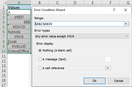
3. 单击“确定”,指定的错误值将根据您所选的选项显示。
Kutools for Excel——通过 300 多款必备工具全面增强 Excel 功能,助您工作更快速、更轻松,并借助 AI 功能实现更智能的数据处理与高效办公!立即获取
使用公式将特定错误替换为其他值
要替换特定的错误值,可借助 Excel 的 IF、IFNA 以及 ERROR.TYPE 函数。但首先,您需了解每种错误值对应的数字代码。
| # Error | 公式 | 返回值 |
| #NULL! | =ERROR.TYPE(#NULL!) | 1 |
| #DIV/0! | =ERROR.TYPE(#DIV/0!) | 2 |
| #VALUE! | =ERROR.TYPE(#VALUE!) | 3 |
| #REF! | =ERROR.TYPE(#REF!) | 4 |
| #NAME? | =ERROR.TYPE(#NAME?) | 5 |
| #NUM! | =ERROR.TYPE(#NUM!) | 6 |
| #N/A | =ERROR.TYPE(#N/A) | 7 |
| #GETTING_DATA | =ERROR.TYPE(#GETTING_DATA) | 8 |
| #SPILL! | =ERROR.TYPE(#SPILL!) | 9 |
| #UNKNOWN! | =ERROR.TYPE(#UNKNOWN!) | 12 |
| #FIELD! | =ERROR.TYPE(#FIELD!) | 13 |
| #CALC! | =ERROR.TYPE(#CALC!) | 14 |
| 其他错误 | =ERROR.TYPE(123) | #N/A |

例如,您有一个如上所示的数值表格。要将“#DIV/0!”错误替换为文本字符串“Divide By Zero Error”,请先找到该错误对应的代码“2”,然后在单元格“B2”中输入以下公式,并向下拖动填充柄,将公式应用到下方的单元格:
=IF(IFNA(ERROR.TYPE(A2),A2)=2,"Divide By Zero Error",A2)
- 在公式中,您可以将错误代码“2”替换为其他错误值对应的代码。
- 在公式中,您可以将文本字符串“Divide By Zero Error”替换为其他提示信息,或替换为“”(空字符串),以将错误显示为空白单元格。
相关文章
在处理 Excel 工作表时,您可能会遇到 #DIV/0、#REF、#N/A 等错误值,这些通常源于公式问题。如何在 Excel 中快速轻松地隐藏所有这些错误值?
如何在 Excel 中将 #DIV/0! 错误替换为更清晰易懂的提示信息?
在 Excel 中使用公式计算时,有时会显示错误信息。例如,公式 =A1/B1 在 B1 为空或为 0 时,会返回 #DIV/0! 错误。有没有办法让这些错误提示更清晰易懂?或者,如果您希望用自定义消息替代这些错误,该如何操作?
当您引用某个单元格时,若被引用的行被删除(如下图所示),该单元格将显示 #REF! 错误。接下来,我将为您介绍如何避免 #REF! 错误,并在删除行时自动引用下一个单元格。
如果您的工作表中包含公式,难免会出现一些错误值。能否一次性高亮显示所有包含错误值的单元格?Excel 的条件格式功能可轻松帮您实现这一需求。
最佳办公效率工具
| 🤖 | KUTOOLS AI 助手:基于以下内容革新数据分析:智能执行 | 生成代码| 创建自定义公式 | 数据分析及生成图表| 调用 Kutools Functions…… |
| 热门功能:查找、高亮或标记重复项 | 删除空白行 | 合并列或单元格且不丢失数据 | 不使用公式的四舍五入…… | |
| 高级 LOOKUP:多条件 VLookup | 多值 VLookup | 跨多工作表 VLookup | 模糊查找…… | |
| 高级下拉列表:快速创建下拉列表 | 级联下拉列表 | 多选下拉列表…… | |
| 列管理器:添加指定数量的列|移动列|切换隐藏列的可见性状态|比较区域与列…… | |
| 特色功能:网格聚焦 | 设计视图 |增强编辑栏 | 工作簿和表管理器 | 资源库(自动文本)| 日期提取 | 汇总工作表 | 加密/解密单元格 | 按列表发送邮件 | 超级筛选 | 特殊筛选(筛选粗体单元格/斜体/删除线……) ...... | |
| 精选 15 工具集:12 文本工具(添加文本,删除特定字符,……)| 50+ 图表 类型(甘特图,……)| 40+ 实用公式(基于生日计算年龄,……)| 19 插入工具(插入二维码,从路径插入图片,……)| 12 转换工具(小写金额转大写,汇率转换,……)| 7 合并和拆分工具(高级合并行,分割单元格,……)|……更多 |
使用 Kutools for Excel 大幅提升您的 Excel 技能,体验前所未有的高效。Kutools for Excel 提供 300 多项高级功能,助您提升生产力、节省时间。立即点击此处,获取您最需要的功能……
Office Tab 为 Office 带来标签式界面,让您的工作更轻松
- 在 Word、Excel、PowerPoint、Publisher、Access、Visio 和 Project 中启用标签式编辑和阅读。
- 在同一个窗口的新标签页中打开并创建多个文档,而非在新窗口中。
- 将您的工作效率提升 50%,每天减少数百次鼠标点击!
所有 Kutools 插件,一个安装程序
Kutools for Office 套件捆绑了适用于 Excel、Word、Outlook 和 PowerPoint 的插件以及 Office Tab Pro,非常适合需要跨多个 Office 应用高效协作的团队。
- 一体化套件— Excel、Word、Outlook 和 PowerPoint 插件 + Office Tab Pro
- 一个安装程序,一个许可证— 几分钟内完成设置(支持 MSI)
- 协同效果更佳— 在多个 Office 应用中实现高效协同
- 30 天全功能试用— 无需注册,无需信用卡
- 超值之选— 比单独购买插件更省钱