如何在 Excel 中将负数快速转换为正数?
在 Excel 中处理数据时,您可能偶尔需要将负数转为正数,或反过来。有没有快捷方法能快速将负数转为正数?本文将为您介绍以下技巧,轻松实现负数与正数之间的相互转换。
使用选择性粘贴函数将负数转换为正数
您可以按照以下步骤将负数转换为正数:
1. 在空白单元格中输入数字 -1,然后选中该单元格,按下 Ctrl+C 进行复制。
2. 选中范围内的所有负数,右键单击,然后从上下文菜单中选择选择性粘贴……。参见截图: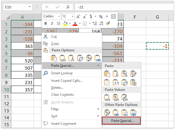
3. 此时将弹出选择性粘贴对话框,在粘贴选项下选择全部,在运算选项下选择乘,然后单击确定。参见截图:
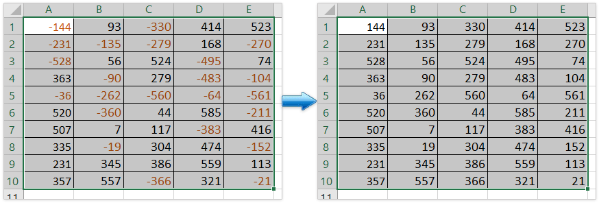
4. 所有选中的负数将被转换为正数,请根据需要删除数字 -1. 效果如图所示:
使用 Kutools for Excel 快速轻松地将负数转换为正数
大多数 Excel 用户不愿使用 VBA 代码,有没有快速将负数转为正数的技巧?Kutools for Excel 助您轻松高效地实现这一目标!
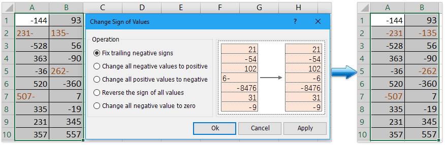
1. 选择包含要更改的负数的区域,然后单击 Kutools > 内容 > 修改数字的符号。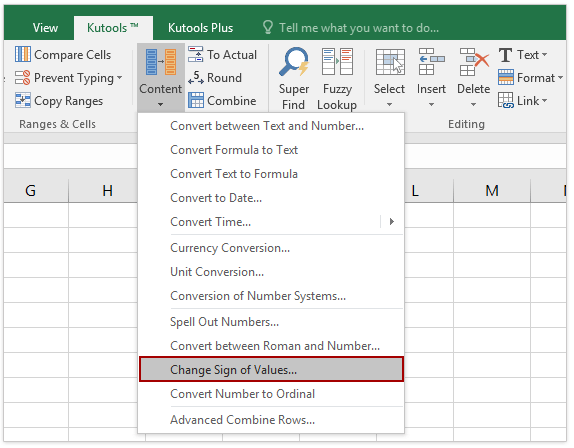
2. 勾选运算下的改变所有的负数为正数选项,然后单击确定。参见截图: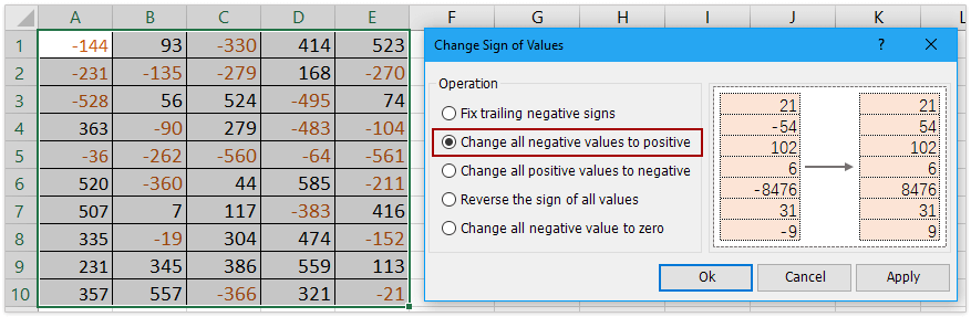
现在您将看到所有负数已变为正数,如下图所示: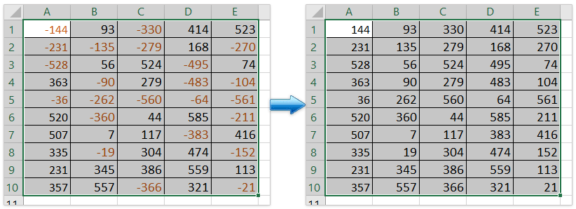

使用 VBA 代码将指定区域内的所有负数转换为正数
作为 Excel 专家,您还可以通过运行 VBA 代码将负数转换为正数。
1. 按下 Alt + F11 键,即可打开 Microsoft Visual Basic for Applications 窗口。
2. 将弹出一个新窗口。单击插入 > 模块,然后在模块中输入以下代码:
Sub Positive
Dim Cel As Range
For Each Cel In Selection
If IsNumeric(Cel.Value) Then
Cel.Value = Abs(Cel.Value)
End If
Next Cel
End Sub3. 然后单击运行按钮或按 F5 键运行程序,即可将所有负数转为正数。效果如图所示:
相关文章
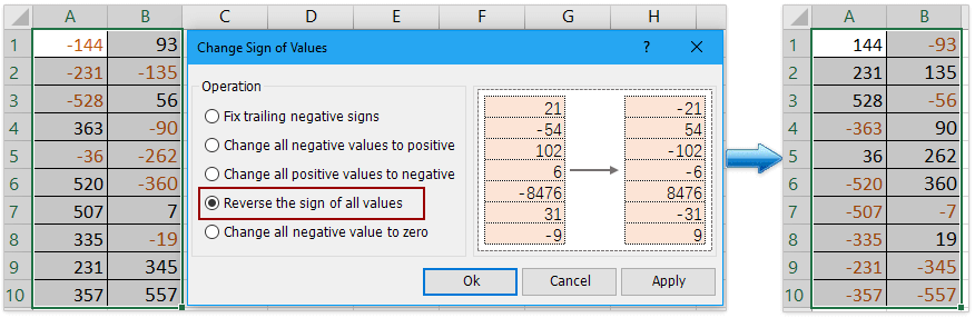
反转单元格中数值的符号
使用 Excel 时,工作表中通常同时包含正数和负数。如果需要将正数变为负数,或将负数转为正数,手动逐个修改固然可行,但面对数百个数据时显然效率低下。有没有更高效的解决方法?
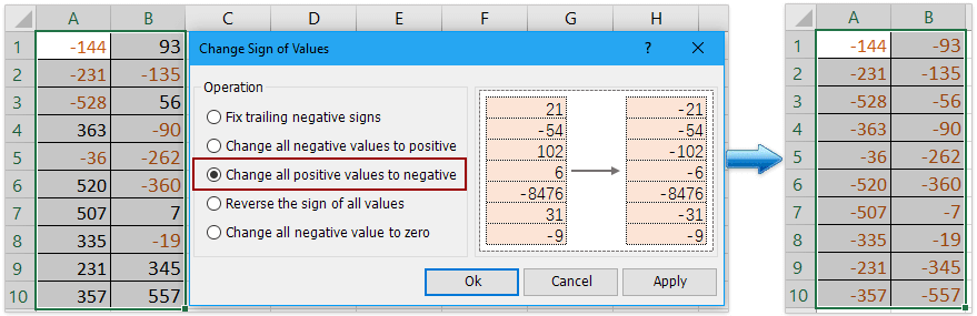
将正数变为负数
如何在 Excel 中快速将所有正数或数值变为负数?以下方法将指导您轻松完成此操作。
修正单元格中所有末尾的负号
出于某些原因,您可能需要在 Excel 中修正单元格中所有末尾的负号。例如,带有尾随负号的数字可能显示为 90——。如何快速将这类负号从右侧移除以修复数据?以下是一些助您高效处理的实用技巧。
将负数更改为零
我将指导您一次性将所选区域中的所有负数轻松更改为零。
该最佳办公效率工具
Kutools for Excel —— 助您脱颖而出
| 🤖 | KUTOOLS AI 助手:基于以下内容革新数据分析:智能执行 | 生成代码| 创建自定义公式 | 数据分析及生成图表| 调用 Kutools Functions…… |
| 热门功能:查找、高亮或标记重复项 | 删除空白行 | 合并列或单元格而不丢失数据 | 不使用公式的四舍五入…… | |
| 超级 VLookup:多条件查询 | 返回多个值 | 跨多工作表查询 | 模糊查找…… | |
| 高级下拉列表:轻松创建下拉列表 | 级联下拉列表 | 多选下拉列表…… | |
| 列管理器:添加指定数量的列 | 移动列 | 切换隐藏列的可见状态 |比较列以选择相同/不同单元格…… | |
| 特色功能:网格聚焦 | 设计视图 | 增强编辑栏 | 工作簿和表管理器|资源库(自动文本)| 日期提取 | 汇总工作表 | 加密/解密单元格 | 按列表发送邮件 | 超级筛选 | 特殊筛选(筛选粗体单元格/斜体/删除线……) ...... | |
| 热门 15 工具集:12 文本工具(添加文本,删除特定字符……)| 50+ 图表 类型(甘特图……)| 40+ 实用公式(基于生日计算年龄……)| 19 插入工具(插入二维码,从路径插入图片……)| 12 转换工具(小写金额转大写,汇率转换……)| 7 合并和拆分工具(高级合并行,拆分 Excel 单元格……)|……更多功能 |
Kutools for Excel 拥有超过 300 项功能,确保您所需的功能触手可及……
Office Tab - 在 Microsoft Office(包括 Excel)中启用标签式阅读与编辑
- 一秒内轻松切换数十个已打开的文档!
- 每天为您省下数百次鼠标点击,轻松告别“鼠标手”。
- 在查看和编辑多个文档时,工作效率提升 50%。
- 为 Office(包括 Excel)带来高效标签页,体验如 Chrome、Edge 和 Firefox 般的流畅操作。