如何在 Excel 中从多列中提取唯一值?
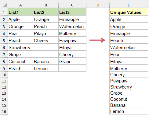
如果您经常在 Excel 中处理跨多列分布的数据集,可能会发现某些值在同一列内或不同列之间重复出现。在许多报表制作或数据分析任务中,识别并提取所有唯一值——即在整个选定区域中仅出现一次的值(无论其位于何处)——往往是必不可少的。手动完成这项工作不仅耗时,还容易出错,尤其在面对大型数据集或复杂表格时更是如此。幸运的是,Excel 提供了多种高效提取这些唯一值的方法。
本指南为您提供了多种解决方案,可根据您使用的 Excel 版本及个人偏好灵活选择——包括适用于所有版本的通用公式、适用于较新版本的动态数组公式、借助 KUTOOLS AI Aide 获得直观结果、利用数据透视表实现可视化整合,以及在复杂场景中通过 VBA 代码完成自动化提取。
使用公式从多列中提取唯一值
有时您可能希望借助 Excel 内置函数来实现这一提取。本节详细介绍了两种方法:一种是适用于所有 Excel 版本的数组公式,另一种则是专为 Excel 365 和 Excel 2021 等较新版本设计的动态数组公式。当您需要直接基于公式的解决方案、要求数据变动时自动更新,或希望避免使用外部加载项或代码时,这些方法尤为理想。
使用适用于所有 Excel 版本的数组公式从多列中提取唯一值
为了兼容所有 Excel 版本,即使您的 Excel 不支持动态数组,也能通过数组公式从多列中提取唯一值。此方法结合了 INDIRECT、TEXT、MIN、IF、COUNTIF、ROW 和 COLUMN函数,轻松适配各种数据结构。
假设您的数据位于 A2:C9 范围内。若要从 E2 单元格开始提取唯一值,请按以下步骤操作:
1. 单击您列表放置区域的第一个单元格(即 )E2),并输入以下数组公式:
=INDIRECT(TEXT(MIN(IF(($A$2:$C$9")*(COUNTIF($E$1:E1,$A$2:$C$9)=0),ROW($2:$9)*100+COLUMN($A:$C),7^8)),"R0C00"),)&""
- A2:C9 是您要提取唯一值的数据区域。
- E1:E1 指的是第一个输出单元格正上方的单元格,用于跟踪哪些条目已被输出。
- $2:$9 是您数据的行引用;$A:$C 是列引用。请根据您的工作表布局灵活调整。
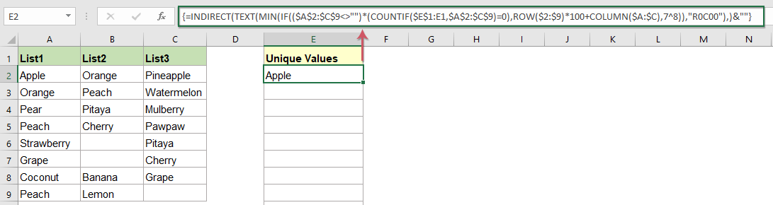
2. 输入公式后,请勿仅按 Enter 键,而应 同时按 Ctrl + Shift + Enter将其确认为数组公式。操作正确时,公式栏中的公式将被花括号 {} 包围。随后,从 E2 向下拖动填充柄,直至出现空白单元格,即表示已无更多唯一值可提取。此操作可确保所有唯一值完整显示在目标列中。

- $A$2:$C$9:请指定用于检查唯一值的完整单元格范围。
- IF(($A$2:$C$9<>"")*(COUNTIF($E$1:E1,$A$2:$C$9)=0), ROW($2:$9)*100+COLUMN($A:$C),7^8):
- $A$2:$C$9<>"" 请确保忽略空白单元格。
- COUNTIF($E$1:E1,$A$2:$C$9)=0 确保仅包含全新的(尚未提取过的)值。
- 当两个条件同时满足时,系统将根据单元格的行号与列号计算出唯一的索引编号。
- 如果任一条件不成立,公式将返回一个非常大的数字()7^8),以避免被意外选中。
- MIN(...)找出最小的索引编号,以精准定位数据中下一个可用唯一值的位置。
- TEXT(...,"R0C00") 将索引转换为采用 R1C1 引用样式的有效单元格引用。
- INDIRECT(...)将上述生成的单元格引用替换为您数据区域中的实际值。
- &““强制将公式结果视为文本,杜绝格式意外。
使用公式从多列中提取唯一值(适用于 Excel 365、Excel 2021 及更新版本)
如果您使用 Excel 365、Excel 2021 或更新版本,即可使用动态数组函数,以更简单、更直观的方式从多列中提取唯一值。UNIQUE 和 TOCOL 函数一步实现跨列数据合并与去重,特别适合处理持续更新或大型数据集的用户。
要使用此方法,只需选择一个空白单元格(例如 )E2,或您希望结果显示的任意位置),输入以下公式,然后按 Enter:
=UNIQUE(TOCOL(A2:C9,1))按 Enter 后,区域 A2:C9 中的所有唯一值将自动溢出到公式下方的单元格中。此功能高效便捷——当源数据发生变化时,输出会动态更新,无需手动刷新!

- TOCOL(A2:C9,1):自动将多列范围内的值转换为单列,并智能剔除空白单元格。
- UNIQUE(...):仅提取每个值一次,生成干净、去重的列表。
使用 KUTOOLS AI Aide 从多列中提取唯一值
如果您希望操作更简便、大幅减少手动操作,KUTOOLS AI Aide(内置于 Kutools for Excel)可轻松帮您从多列中提取唯一值。对于不熟悉公式或希望避免公式出错的用户来说,这一功能尤为实用。KUTOOLS AI Aide 能准确理解您的指令并自动处理数据,无论您是初学者,还是只想通过几次点击快速解决问题,都能得心应手。
安装后,单击 KUTOOLS AI>AI 助手 以打开“KUTOOLS AI Aide”窗格:
- 在聊天框中输入您的请求,例如:“从范围 A2:C9 中提取唯一值(忽略空白单元格),并将结果从 E2 开始放置:”
- 点击“发送”或按 Enter 键,AI 分析请求后,只需点击“执行”即可立即运行,结果将出现在您指定的工作表位置。
提示:如果您的数据提取流程经常变动,或希望使用自然语言处理功能,此解决方案尤为实用。若原始数据不够规范,请务必在提取列表中检查空单元格——因为空白条目可能会根据您的 AI 请求细节被包含或过滤。

使用数据透视表从多列中提取唯一值
数据透视表是另一种便捷提取唯一值的方法,尤其适合偏好使用可视化工具,并希望对唯一项进行汇总或进一步分析(例如统计出现次数)的用户。该方法简单直接,无需使用公式,但需完成若干设置步骤,并对数据稍作调整——特别是当涉及的列标题不一致时。
以下是使用数据透视表提取唯一值的建议流程:
1. 立即在数据左侧插入一个新空白列。例如,如果您的数据从 B 列开始,则插入新的 A 列。此调整有助于确保合并范围准确无误。

2. 选择数据集中的任意单元格,按下 Alt + D 后迅速按 P,即可启动“数据透视表和数据透视图向导”。在向导第一步中,选择“多重合并计算区域”,即可将多个列中的值合并到一个汇总字段中。

3. 单击下一步,然后选择“为我创建单页字段”。此步骤会将所有数据整合为一个组,便于提取唯一值。

4. 在下一步中,选择整个数据区域(包括新插入的空白列),点击添加按钮,将所选内容加入“所有区域”列表,然后单击下一步。

5. 在向导的最后一步中,选择您希望放置数据透视表的位置(新工作表或现有工作表),然后单击完成,即可生成数据透视表报告。

6. 在新生成的数据透视表中,取消勾选“选择要添加到报表的字段”区域中的所有字段,即可清除默认视图。

7. 最后,将“值”字段拖到行区域,数据透视表便会以整洁的单列形式展示原始多列范围中的所有唯一值。

局限性:数据需要预先整理,且当您的源数据更新时,必须刷新数据透视表才能看到新的唯一值。
使用 VBA 代码从多列中提取唯一值
在需要自动化提取或处理大型且不规则数据集时,使用 VBA(Visual Basic for Applications)代码可提供一种快速、可重复的解决方案。该方法特别适合具备 Excel VBA 编辑器基础知识的用户,或希望在重复性任务中最大限度减少手动操作的场景。与数组公式相比,VBA 在处理大量数据时也更为高效。
1. 按 Alt + F11 打开 VBA 编辑器。在弹出的“Microsoft Visual Basic for Applications”窗口中,单击插入 > 模块,即可添加新模块。
2. 在新模块中粘贴以下代码:
VBA:从多列中提取唯一值
Sub Uniquedata()
'Updateby Extendoffice
Dim rng As Range
Dim InputRng As Range, OutRng As Range
Set dt = CreateObject("Scripting.Dictionary")
xTitleId = "KutoolsforExcel"
Set InputRng = Application.Selection
Set InputRng = Application.InputBox("Range :", xTitleId, InputRng.Address, Type:=8)
Set OutRng = Application.InputBox("Out put to (single cell):", xTitleId, Type:=8)
For Each rng In InputRng
    If rng.Value <> "" Then
        dt(rng.Value) = ""
    End If
Next
OutRng.Range("A1").Resize(dt.Count) = Application.WorksheetFunction.Transpose(dt.Keys)
End Sub
3. 按 F5 运行代码,系统将弹出对话框提示您选择数据区域。请选择所有相关列(包括含空单元格的列)。

4. 单击确定后,系统将再次提示您指定唯一值的输出位置。请指定一个上方的单元格作为结果列表的起始位置(例如,)E2)。

5. 单击“确定”后,宏将自动运行,所有唯一值将从您指定的位置开始显示。

- 如果使用公式时出现 #VALUE!或 #SPILL!等错误,请检查所选范围,并确保输出区域为空,以免影响计算结果。
- 请始终检查您的数据区域中是否存在隐藏行或合并单元格,因为这些都可能影响唯一值提取的准确性。
- 数组公式和动态数组公式会随数据变化自动更新,而高级筛选与数据透视表则可能需要手动刷新或重新运行。
- 对于重复性任务,建议使用 VBA 实现自动化提取,以确保高效一致、精准提速。
- 在应用任何批量提取或自动化操作前,请务必备份您的数据,尤其是在处理复杂工作簿时。
更多相关文章:
- 统计列表中唯一值和不同值的数量
- 假设您有一个包含重复项的长列表,希望统计某一列中唯一值(即仅出现一次的值)或不同值的总数,如左侧截图所示。本文将为您介绍在 Excel 中高效统计唯一值与不同值的方法。
- 在 Excel 中根据条件提取唯一值
- 假设您希望根据 A 列中的特定条件,仅从 B 列中提取唯一名称,并获得如截图所示的结果。本教程将为您演示如何在提取唯一值时应用条件筛选。
- 在 Excel 中仅允许输入唯一值
- 如果您希望在工作表列中仅允许输入唯一值,防止重复项出现,本文将为您介绍在 Excel 中轻松实施唯一性规则的实用技巧。
- 在 Excel 中根据条件对唯一值求和
- 例如,您可能需要根据相邻列中的名称,仅对“订单”列中的唯一值进行求和,如截图所示。本文将探讨如何结合唯一值与条件进行计算。
最佳办公效率工具
| 🤖 | KUTOOLS AI 助手:基于以下内容革新数据分析:智能执行 | 生成代码| 创建自定义公式 | 数据分析及生成图表| 调用 Kutools Functions…… |
| 热门功能:查找、高亮或标记重复项 | 删除空白行 | 合并列或单元格且不丢失数据 | 不使用公式的四舍五入…… | |
| 高级 LOOKUP:多条件 VLookup | 多值 VLookup | 跨多工作表 VLookup | 模糊查找…… | |
| 高级下拉列表:快速创建下拉列表 | 级联下拉列表 | 多选下拉列表…… | |
| 列管理器:添加指定数量的列|移动列|切换隐藏列的可见性状态|比较区域与列…… | |
| 特色功能:网格聚焦 | 设计视图 |增强编辑栏 | 工作簿和表管理器 | 资源库(自动文本)| 日期提取 | 汇总工作表 | 加密/解密单元格 | 按列表发送邮件 | 超级筛选 | 特殊筛选(筛选粗体单元格/斜体/删除线……) ...... | |
| 精选 15 工具集:12 文本工具(添加文本,删除特定字符,……)| 50+ 图表 类型(甘特图,……)| 40+ 实用公式(基于生日计算年龄,……)| 19 插入工具(插入二维码,从路径插入图片,……)| 12 转换工具(小写金额转大写,汇率转换,……)| 7 合并和拆分工具(高级合并行,分割单元格,……)|更多功能 |
Kutools for ExcelKutools for Excel 提供 300 多项高级功能,助您大幅提升生产力并节省时间。立即点击获取您最需要的功能……
Office Tab 为 Office 带来标签式界面,让您的工作更加轻松
- 在 Word、Excel、PowerPoint、Publisher、Access、Visio 和 Project 中启用标签式编辑与阅读,大幅提升多文档操作效率!
- 在同一个窗口的新标签页中打开并创建多个文档,而非在新窗口中操作。
- 将您的工作效率提升 50%,每天减少数百次鼠标点击!
所有 Kutools 插件,一个安装程序
Kutools for Office 套件集成了 Excel、Word、Outlook 和 PowerPoint 插件以及 Office Tab Pro,是跨多个 Office 应用高效协作团队的理想之选。
- 一体化套件— Excel、Word、Outlook 和 PowerPoint 插件 + Office Tab Pro
- 一个安装程序,一个许可证— 几分钟内完成设置(支持 MSI)
- 协同效果更佳— 在多个 Office 应用中实现高效协同办公
- 30 天全功能试用— 无需注册,无需信用卡
- 超值之选— 比单独购买各插件更省钱