在 Excel 中自动高亮显示活动行和列(完整指南)
在包含大量数据的 Excel 工作表中导航颇具挑战,稍不留神就容易迷失位置或误读数值。为助您更高效地分析数据并显著降低出错几率,我们为您介绍 3 种方法,可动态高亮显示 Excel 中所选单元格所在的行与列。当您在不同单元格间移动时,高亮区域将实时跟随变化,提供清晰直观的视觉指引,确保您始终聚焦于正确的数据,效果如下方演示所示:
在 Excel 中自动高亮显示活动行和活动列
- 使用 VBA 代码-清除现有单元格颜色,不支持撤销操作
- 只需单击一次 Kutools for Excel-保留现有单元格颜色,支持撤销操作,适用于受保护的工作表
- 使用使用条件格式-在大数据量下不稳定,需手动刷新(F9)
使用 VBA 代码自动高亮显示活动行和活动列
以下 VBA 代码可助您在当前工作表中自动高亮显示所选单元格所在的整行与整列。
步骤 1:打开要启用自动高亮活动行和列的工作表
步骤 2:打开 VBA 工作表模块编辑器并复制代码
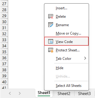
- 右键单击工作表名称,从上下文菜单中选择“查看代码”,参见截图:
- 在打开的 VBA 工作表模块编辑器中,将以下代码复制并粘贴到空白模块中。参见截图:
VBA 代码:自动高亮显示所选单元格的行和列Private Sub Worksheet_SelectionChange(ByVal Target As Range) 'Update by Extendoffice Dim rowRange As Range Dim colRange As Range Dim activeCell As Range Set activeCell = Target.Cells(1, 1) Set rowRange = Rows(activeCell.Row) Set colRange = Columns(activeCell.Column) Cells.Interior.ColorIndex = xlNone rowRange.Interior.Color = RGB(248, 150, 171) colRange.Interior.Color = RGB(173, 233, 249) End Sub提示:自定义代码- 要更改高亮颜色,只需修改以下脚本中的 RGB 值即可:
rowRange.Interior.Color = RGB(248, 150, 171)
colRange.Interior.Color = RGB(173, 233, 249) - 若仅高亮所选单元格的整行,请删除或注释掉(在行首添加单引号)以下代码行:
colRange.Interior.Color = RGB(173, 233, 249) - 若仅高亮所选单元格的整列,请删除或注释掉(在行首添加单引号)以下代码行:
rowRange.Interior.Color = RGB(248, 150, 171)

- 要更改高亮颜色,只需修改以下脚本中的 RGB 值即可:
- 随后,关闭 VBA 编辑器窗口,返回工作表。


效果:
现在,当您选择某个单元格时,该单元格的整行和列会自动高亮显示,并随着所选单元格的变化而动态更新,如下方演示所示:
- 此代码将清除工作表中所有单元格的背景色,因此,若您的单元格包含自定义着色,请勿使用此解决方案。
- 运行此代码将禁用工作表中的“撤销”功能,您将无法通过“Ctrl + Z”快捷键撤消任何误操作。
- 此代码无法在受保护的工作表中运行。
- 要停止高亮所选单元格的行和列,请删除之前添加的 VBA 代码,然后依次点击“开始” > “填充颜色” > “无填充”,即可清除高亮效果。
通过单击一次 Kutools 自动高亮显示活动行和活动列
是否感受到 Excel 中 VBA 代码的局限性?“Kutools for Excel”的“网格聚焦”功能正是您的理想之选!专为弥补 VBA 的不足而打造,提供丰富多样的高亮样式,全面升级您的表格使用体验。更可将这些样式一键应用至所有已打开的工作簿,让数据管理始终高效流畅,视觉效果出众。
安装 Kutools for Excel 后,请单击“Kutools”>“网格聚焦”以启用该功能。启用后,活动单元格所在的行和列将立即高亮显示,并随您切换单元格选择而动态更新。效果如下所示:
- 保留原始单元格背景颜色:
与 VBA 代码不同,此功能会尊重您工作表中已有的格式设置。 - 可在受保护的工作表中使用:
该功能在工作表受保护时仍可无缝运行,非常适合在确保安全性的同时高效管理敏感或共享文档。 - 不影响撤销功能:
使用此功能,您可完全保留 Excel 的撤销功能,轻松撤消更改,为数据操作增添一层安全保障。 - 在处理大型数据时性能稳定:
该功能专为高效处理大型数据集而设计,即使面对复杂且数据密集的电子表格,也能确保稳定流畅的性能表现。 - 多种高亮样式:
此功能提供丰富的高亮选项,您可从多种样式与颜色中自由选择,让活动单元格所在的行、列或行列以最符合您偏好和需求的方式醒目突出。

- 要禁用此功能,请再次点击“Kutools” > “网格聚焦”以关闭该功能;
- 要使用此功能,请 下载并安装 Kutools for Excel。
使用使用条件格式自动高亮显示活动行和活动列
在 Excel 中,您还可以通过设置条件格式,自动高亮显示活动行和活动列。请按以下步骤操作:
步骤 1:选择数据区域
首先,选择要应用此功能的单元格区域——可以是整个工作表,也可以是特定数据集。这里我将选择整个工作表。
步骤 2:进入使用条件格式
单击“开始”>“使用条件格式”>“新建规则”,参见截图:
步骤 3:在“新建格式规则”中设置操作
- 在“新建格式规则”对话框中,从“选择规则类型”列表框中选择“使用公式确定要设置格式的单元格”。
- 在“为符合此公式的值设置格式”框中,输入以下任一公式。本例中,我将使用第三个公式,高亮显示活动行和活动列。
高亮显示活动行:
高亮显示活动列:=CELL("row")=ROW()
高亮显示活动行和活动列:=CELL("col")=COLUMN()=OR(CELL("row")=ROW(), CELL("col")= COLUMN()) - 然后,单击“格式”按钮。

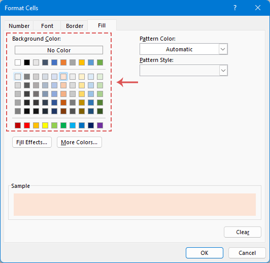
- 在随后弹出的“设置单元格格式”对话框中,切换到“填充”选项卡,选择一种颜色以高亮显示活动行和活动列,参见截图:
- 随后,依次单击“确定” > “确定”,即可关闭对话框。


效果:
现在,A1 单元格所在的整列和整行已同步高亮显示。若要将此高亮效果应用到其他单元格,只需单击目标单元格,然后按“F9”键刷新工作表,即可高亮显示新选中单元格所在的整列与整行。
- 确实,虽然在 Excel 中使用使用条件格式方法进行高亮是一种解决方案,但不如使用“VBA”和“网格聚焦”功能那样流畅。此方法需要手动重新计算工作表(通过按“F9”键实现)。
要启用工作表的自动重新计算功能,您可以将一段简单的 VBA 代码插入到目标工作表的代码模块中。这将自动执行刷新过程,确保在您选择不同单元格时立即更新高亮效果,而无需按“F9”键。请右键单击工作表名称,然后从上下文菜单中选择“查看代码”。然后将以下代码复制并粘贴到工作表模块中:Private Sub Worksheet_SelectionChange(ByVal Target As Range) Target.Calculate End Sub - 使用条件格式时,您手动应用于工作表的现有格式将被保留。
- 条件格式以易变性著称,尤其在处理超大型数据集时更是如此。过度使用可能拖慢工作簿性能,影响数据处理与导航效率。
- CELL 函数仅适用于 Excel 2007 及更高版本,与早期版本的 Excel 不兼容。
上述方法对比
| 功能 | VBA 代码 | 使用条件格式 | Kutools for Excel |
| 保留单元格背景颜色 | 否 | 是 | 是 |
| 支持撤销 | 否 | 是 | 是 |
| 在大型数据集中运行稳定 | 否 | 否 | 是 |
| 可在受保护的工作表中使用 | 否 | 是 | 是 |
| 适用于所有打开的工作簿 | 仅当前工作表 | 仅当前工作表 | 所有打开的工作簿 |
| 需要手动刷新(F9) | 否 | 是 | 否 |
以上就是在 Excel 中高亮显示所选单元格所在行和列的完整指南。如果您想探索更多 Excel 使用技巧,我们网站提供了数千篇实用教程,请点击此处访问。感谢您的阅读,期待未来继续为您带来更多精彩内容!
相关文章:
- 自动高亮显示活动单元格所在的行和列
- 当您浏览包含大量数据的工作表时,不妨高亮显示所选单元格所在的行和列,让数据阅读更轻松、直观,有效避免误读。接下来,我将为您介绍一些实用技巧:在当前单元格中高亮显示活动单元格的行和列,并在单元格切换时,自动高亮新单元格所在的行与列。
- 在 Excel 中高亮显示每隔一行或一列
- 在大型工作表中,为每隔一行(或第 n 行)或一列(或第 n 列)添加高亮或填充色,可显著提升数据的可见性与可读性。这不仅让工作表更整洁美观,还能助您更快掌握数据要点。本文将为您介绍多种为每隔一行(或第 n 行)或一列(或第 n 列)着色的方法,让您的数据呈现更清晰、更具吸引力。
- 滚动时高亮整行
- 如果您的工作表包含多列数据,滚动时可能难以分辨某一行中的内容。此时,不妨高亮显示活动单元格所在的整行,这样在水平滚动时就能快速、轻松地追踪该行数据。本文将为您介绍几种实用技巧,助您轻松解决这一难题。
- 根据下拉列表进行高亮行区域
- 本文将介绍如何根据下拉列表选项高亮整行区域。以下图为例:当在 E 列的下拉列表中选择“进行中”时,该行将以红色高亮显示;选择“已完成”时,以蓝色高亮显示;选择“未开始”时,则以绿色高亮显示该行。
最佳办公效率工具
| 🤖 | KUTOOLS AI 助手:基于以下内容革新数据分析:智能执行 | 生成代码| 创建自定义公式 | 数据分析及生成图表| 调用 Kutools Functions…… |
| 热门功能:查找、高亮或标记重复项 | 删除空白行 | 合并列或单元格而不丢失数据 | 不使用公式的四舍五入…… | |
| 高级 LOOKUP:多条件 VLookup | 多值 VLookup | 跨多工作表 VLookup | 模糊查找…… | |
| 高级下拉列表:快速创建下拉列表 | 级联下拉列表 | 多选下拉列表…… | |
| 列管理器:添加指定数量的列|移动列|切换隐藏列的可见性状态|比较区域与列…… | |
| 特色功能:网格聚焦 | 设计视图 |增强编辑栏 | 工作簿和表管理器 | 资源库(自动文本)| 日期提取 | 汇总工作表 | 加密/解密单元格 | 按列表发送邮件 | 超级筛选 | 特殊筛选(筛选粗体单元格/斜体/删除线……) ...... | |
| 顶级 15 工具集:12 文本工具(添加文本,删除特定字符,……)| 50+ 图表 类型(甘特图,……)| 40+ 实用公式(基于生日计算年龄,……)| 19 插入工具(插入二维码,从路径插入图片,……)| 12 转换工具(小写金额转大写,汇率转换,……)| 7 合并和拆分工具(高级合并行,分割单元格,……)|……以及更多 |
Kutools for ExcelKutools for Excel 提供超过 300 项高级功能,助您显著提升工作效率并节省时间。立即点击,获取您最需要的功能……
Office Tab 为 Office 带来标签式界面,让您的工作更加轻松
- 在 Word、Excel、PowerPoint、Publisher、Access、Visio 和 Project 中启用标签式编辑与阅读,大幅提升多文档操作效率!
- 在同一个窗口的新标签页中打开并创建多个文档,无需开启新窗口。
- 每天为您省下数百次鼠标点击,工作效率提升 50%!
所有 Kutools 插件,一个安装程序
Kutools for Office 套件整合了 Excel、Word、Outlook 和 PowerPoint 插件,以及 Office Tab Pro,非常适合需要跨多个 Office 应用高效协作的团队使用。
- 一体化套件— Excel、Word、Outlook 与 PowerPoint 插件 + Office Tab Pro
- 一个安装程序,一个许可证— 几分钟内完成设置(支持 MSI)
- 协同效果更佳— 在多个 Office 应用中实现高效流畅的办公体验
- 30 天全功能试用— 无需注册,无需信用卡
- 超值之选— 比单独购买各插件更省钱