如何在Excel中vlookup值并返回true或false / yes或no?
在许多情况下,您可能需要在一列中查找值,如果在另一列中是否找到该值,则只返回true或false(是或否)。 在本文中,我们将向您展示实现该目标的方法。
Vlookup并使用公式返回true或false / yes或no
如果使用出色的工具在另一列中找到值,则突出显示该列中的值
有关VLOOKUP的更多教程...
Vlookup并使用公式返回true或false / yes或no
假设您具有范围A2:A18中的数据列表,如以下屏幕截图所示。 要根据D2:D18中的值搜索A2:A4中的值并显示结果True或false / Yes或No,请执行以下操作。

1.选择一个空白单元格以输出结果。 在这里,我选择B2。
2.在其中输入以下公式,然后按 输入 键。
=IF(ISNA(VLOOKUP(A2,$D$2:$D$4,1,FALSE)), "No", "Yes")
3.选择结果单元格,然后拖动“填充手柄”以将公式应用于其他单元格(在这种情况下,我向下拖动“填充手柄”,直到达到B18)。 看截图:

请注意: 要返回True或False,请用“ True”和“ False”替换公式中的“是”和“否”:
=IF(ISNA(VLOOKUP(A2,$D$2:$D$4,1,FALSE)), "False", "True")

如果使用出色的工具在另一列中找到值,则突出显示该列中的值
如果您想在另一列中突出显示某个值(例如用背景色突出显示它们),则强烈建议您使用 选择相同和不同的单元格 实用程序 Kutools for Excel。 使用此实用程序,您只需单击即可轻松实现。 如下面的演示所示。 立即下载 Kutools for Excel! (30 天免费试用)
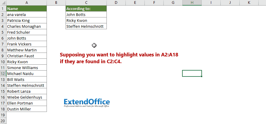
让我们看看如果在另一列中找到值,如何应用此功能突出显示一列中的值。
1. 安装 Kutools for Excel 后,单击 库工具 > 选择 > 选择相同和不同的单元格 启用该实用程序。

2.在 选择相同和不同的单元格 对话框,请进行以下配置。
- 2.1)在 在中查找值 框中,选择要突出显示值的范围;
- 2.2)在 根据 框,选择将突出显示值的范围;
- 2.3)在 基于 部分,检查 单细胞 选项;
- 2.4)在 找到最适合您的地方 部分,选择 相同的值 选项;
- 2.5)在 处理结果 部分,检查 填充背景色 or 填充字体颜色 根据需要指定突出显示颜色;
- 2.6)点击 OK 按钮。 看截图:

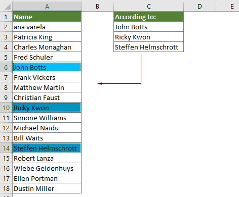
然后,如果在C2:C18中找到了范围A2:A4中的值,它们将被突出显示并立即选择,如下面的屏幕截图所示。
如果您想免费试用(30天)此实用程序, 请点击下载,然后按照上述步骤进行操作。
相关文章
跨多个工作表的Vlookup值
您可以应用vlookup函数以返回工作表中的匹配值。 但是,如果您需要在多个工作表中使用vlookup值,该怎么办? 本文提供了详细的步骤来帮助您轻松解决问题。
Vlookup并在多列中返回匹配的值
通常,应用Vlookup函数只能从一列返回匹配的值。 有时,您可能需要根据条件从多个列中提取匹配的值。 这是您的解决方案。
Vlookup在一个单元格中返回多个值
通常,应用VLOOKUP函数时,如果存在多个符合条件的值,则只能获取第一个的结果。 如果要返回所有匹配的结果并将它们全部显示在一个单元格中,如何实现?
Vlookup并返回匹配值的整个行
通常,使用vlookup函数只能返回同一行中特定列的结果。 本文将向您展示如何根据特定条件返回整行数据。
向后Vlookup或反向
通常,VLOOKUP函数在数组表中从左到右搜索值,并且它要求查找值必须位于目标值的左侧。 但是,有时您可能知道目标值,并想找出相反的查找值。 因此,您需要在Excel中向后vlookup。 本文中有几种方法可以轻松解决此问题!
最佳办公生产力工具
| 🤖 | Kutools 人工智能助手:基于以下内容彻底改变数据分析: 智能执行 | 生成代码 | 创建自定义公式 | 分析数据并生成图表 | 调用 Kutools 函数... |
| 热门特色: 查找、突出显示或识别重复项 | 删除空白行 | 合并列或单元格而不丢失数据 | 不使用公式进行四舍五入 ... | |
| 超级查询: 多条件VLookup | 多值VLookup | 跨多个工作表的 VLookup | 模糊查询 .... | |
| 高级下拉列表: 快速创建下拉列表 | 依赖下拉列表 | 多选下拉列表 .... | |
| 列管理器: 添加特定数量的列 | 移动列 | 切换隐藏列的可见性状态 | 比较范围和列 ... | |
| 特色功能: 网格焦点 | 设计图 | 大方程式酒吧 | 工作簿和工作表管理器 | 资源库 (自动文本) | 日期选择器 | 合并工作表 | 加密/解密单元格 | 按列表发送电子邮件 | 超级筛选 | 特殊过滤器 (过滤粗体/斜体/删除线...)... | |
| 前 15 个工具集: 12 文本 工具 (添加文本, 删除字符,...) | 50+ 图表 类型 (甘特图,...) | 40+ 实用 公式 (根据生日计算年龄,...) | 19 插入 工具 (插入二维码, 从路径插入图片,...) | 12 转化 工具 (小写金额转大写, 货币兑换,...) | 7 合并与拆分 工具 (高级组合行, 分裂细胞,...) | ... 和更多 |
使用 Kutools for Excel 增强您的 Excel 技能,体验前所未有的效率。 Kutools for Excel 提供了 300 多种高级功能来提高生产力并节省时间。 单击此处获取您最需要的功能...
")
Office Tab 为 Office 带来选项卡式界面,让您的工作更加轻松
- 在Word,Excel,PowerPoint中启用选项卡式编辑和阅读,发布者,Access,Visio和Project。
- 在同一窗口的新选项卡中而不是在新窗口中打开并创建多个文档。
- 每天将您的工作效率提高50%,并减少数百次鼠标单击!
")